General introduction
This is chapter 1 of my PhD thesis, defended at Radboud University in . It was written for the thesis and has not been published elsewhere.
Overview & epidemiology
On average, one in nine men gets diagnosed with prostate cancer during their lifetime. With more than 1.2 million new cases each year,1 prostate cancer is the second most common cancer among men. The incidence of prostate cancer is steadily increasing, and as prostate cancer is mostly associated with advancing age,2 the WHO expects that there will be 2.3 million new patients yearly by 2040.3
In the Netherlands specifically, the statistics show the same trend. Yearly, around 14.000 men are diagnosed with prostate cancer for the first time,4 making it the most common cancer among men in the Netherlands. Compared to only 4.000 new cases in 1989, prostate cancer incidence is increasing steadily due to an aging population and an increase in testing (Figure 1.1).
With an estimate of 350.000 deaths per year globally, prostate cancer has a high incidence-to-mortality ratio and co-occurs with an increased risk of overdiagnosis and overtreatment.5 Over time, the mortality rate decreased, but we still see a rise in absolute mortality due to a sharp increase in prostate cancer incidence.
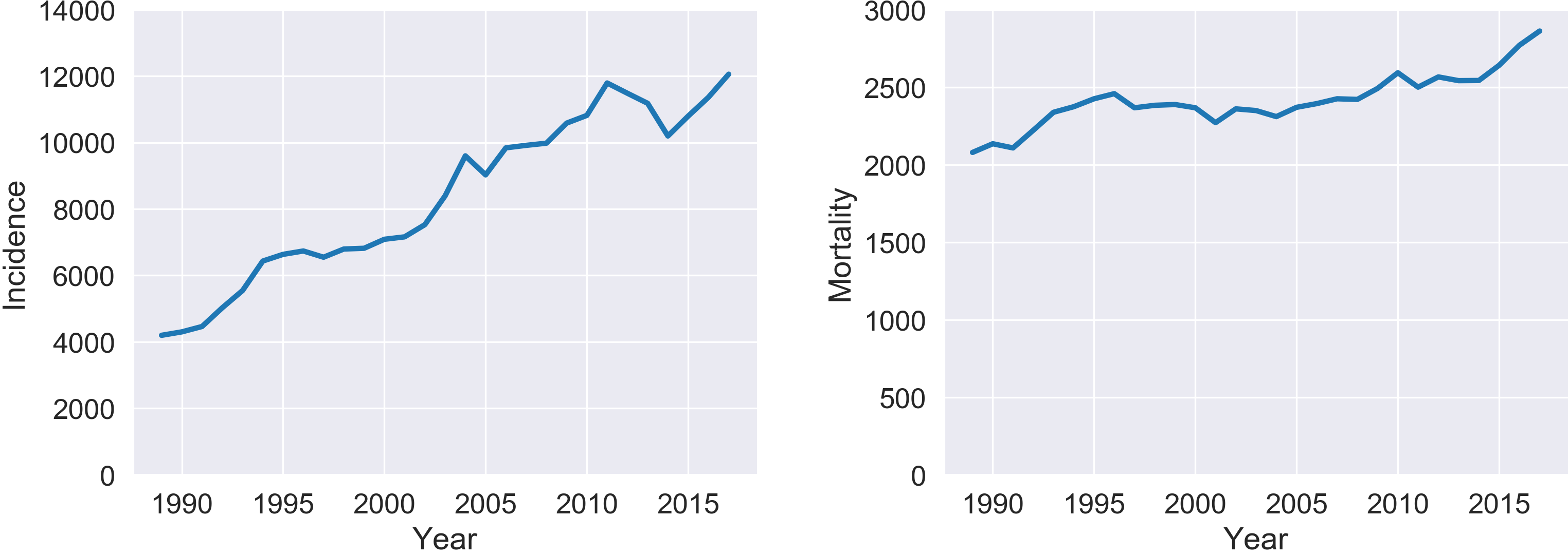
Absolute incidence (left) and mortality (right) of prostate cancer within the Netherlands from 1989 to 2017.4
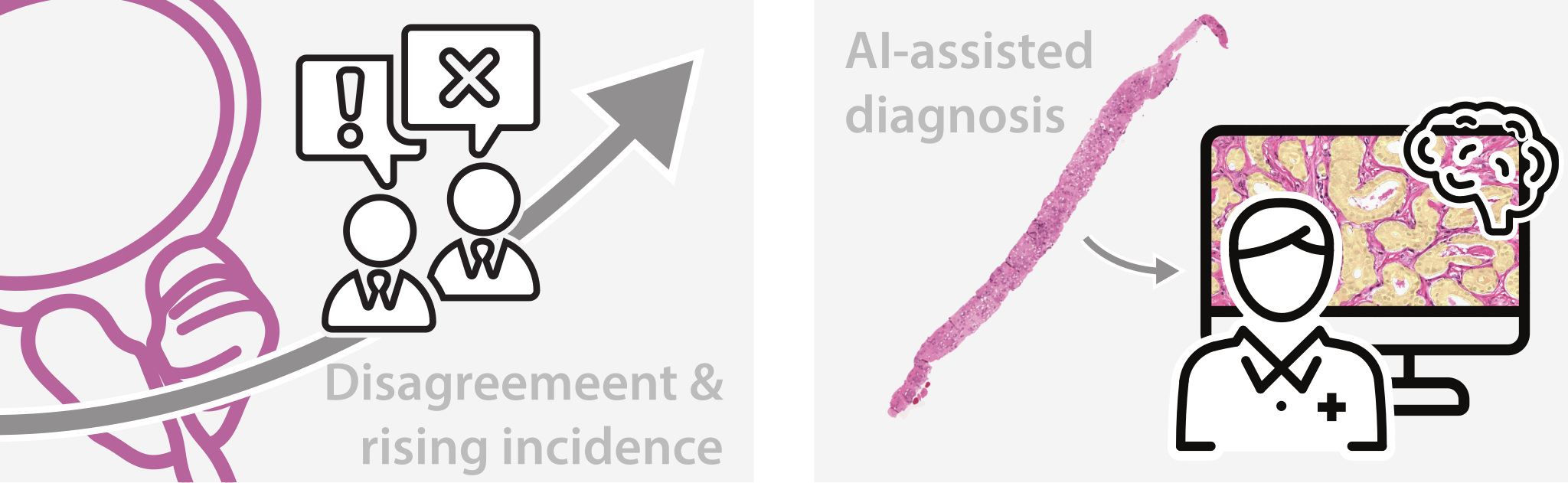
The risks of overdiagnosis and overtreatment stress the need for an accurate diagnosis of prostate cancer. The key to diagnosing prostate cancer is the histological assessment of prostate tissue by pathologists. Unfortunately, this process suffers from considerable inter- and intraobserver variability. Artificial intelligence (AI) systems could assist pathologists in diagnosing prostate cancer due to their ability to learn patterns from data effectively. This thesis will cover the development, validation, and evaluation of the potential of AI algorithms to improve prostate cancer diagnosis in histological tissue sections (Figure 1.2).
Prostate cancer
Prostate anatomy
The prostate is a small organ located in the male pelvis (Figure 1.3, left), just below the bladder, and surrounds the urethra. The prostate is part of the male reproductive system, and its function is to secrete a fluid that will contribute to the total volume of the semen and prolong the spermatozoa’s lifespan. Around 30% of the semen consists of prostatic fluid. Muscle cells within the prostate help with the secretion of the semen during ejaculation.
In pathology, the prostate is most commonly divided into three distinct zones: the peripheral, central, and transition zone (Figure 1.3, right). The peripheral zone is the largest, with around 70% of the glandular tissue, and resides at the back of the prostate. The large majority of prostate cancers originate from the peripheral zone.67 The central zone consists of around 25% of the tissue and surrounds the urethra. Despite its size, the central zone only accounts for around 2.5% of prostate cancers.6 Finally, the transition zone occupies approximately 20% of the tissue and 20% of the found prostate cancers.68
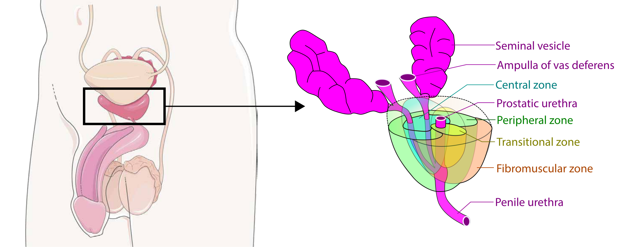
Anatomy of the male reproductive system (left) with the prostate outlined, and a schematic overview of the prostatic zones (right). Prostate anatomy illustration by Servier Medical Art, CC BY 4.0; zones diagram by Mikael Häggström, CC0, via Wikimedia Commons.
Current diagnostic pathway
The possible presence of prostate cancer can be detected using a blood test, which measures the concentration of prostate-specific antigen (PSA) in the blood. PSA is mainly secreted by the epithelial cells within the prostate, and an increase in the number of cells will result in an elevated PSA level. Unfortunately, a high PSA value is not specific to prostate cancer as benign disorders can also elevate the PSA concentration.
Due to the low specificity, screening for prostate cancer using PSA measurements is highly controversial. As an illustration, results of the European Randomized Study of Screening for Prostate Cancer showed that, after a median follow-up of nine years, to save one life, 1410 men would need to be screened, and 48 additional cases of prostate cancer would need to be treated.9 These numbers become more favorable with longer follow-up times.510
So, while PSA screening could result in a significant decrease in mortality, it would also introduce additional overdiagnosis and overtreatment. It is therefore important to not only look at mortality reduction, but also take quality of life (QALYs) into account given the high side effects of treatment.11 In the Netherlands, there is no screening program for prostate cancer as it is expected that it would lead to drastic overtreatment.12 Additionally, due to the risk of overdiagnosis, general practitioners are advised to discuss the downsides of performing a PSA test with patients.13
Although there is no official PSA screening program in The Netherlands, a PSA test is often still the first step in the diagnostic pathway of prostate cancer. The PSA test is commonly combined with a digital rectal examination (DRE) by a urologist. When there is a further confirmed suspicion of prostate cancer, traditionally, the next step would be to take systematic transrectal ultrasound-guided (TRUS) biopsies. During this procedure, eight to twelve biopsies are taken from different regions in the prostate guided by an ultrasound probe.14 It has been shown that taking twelve biopsies increases the cancer detection rate, but the TRUS biopsies still have limited sensitivity for prostate cancer.1516
With advances in imaging techniques, it recently became a new standard in the Netherlands to perform an MRI scan before a biopsy procedure to reduce the number of invasive biopsy procedures.17 Still, to fully confirm the presence of prostate cancer, histological assessment of the tissue is required. If the MRI is positive, it is advised to perform an MRI-guided biopsy procedure, with optionally additional systematic biopsies. The combination of MRI-guided and systematic biopsies has been shown to be more specific.16 If the MRI was negative, in consultation with the patient, a further biopsy procedure can be omitted.
Histology
After a prostate biopsy is taken, the sample is sent for histopathological assessment by a pathologist. Histopathology is the medical science that studies the microscopic structures of tissue (histology) to understand human diseases (pathology). In clinical diagnostics, pathologists analyze samples of human tissue using bright-field microscopy in order to determine a diagnosis for the patient.
After the biopsy procedure, whether TRUS-, MRI-guided or systematic, the specimen cannot be directly examined by pathologists. The tissue is first fixated to prevent decay by immersing the sample in formalin; this ensures that the sample can be preserved for extended periods. After fixation, any remaining water is removed, and the sample is embedded in paraffin (FFPE, formalin-fixed paraffin-embedded). From this embedded block, very thin sections can be cut using a microtome—typically only a few micrometers thick. After cutting, the sections are mounted on glass slides for easier handling and to enable microscopic inspection.
When mounted, a staining procedure is applied to highlight specific parts of the tissue. The most common staining procedure worldwide stains tissue using hematoxylin and eosin (H&E), with hematoxylin staining nuclear DNA in blue and eosin staining cytoplasmic and tissue proteins in shades of pink (Figure 1.4). Between labs, or even within the same lab, the exact color characteristics can vary drastically due to (small) differences in the procedures and environmental influences.
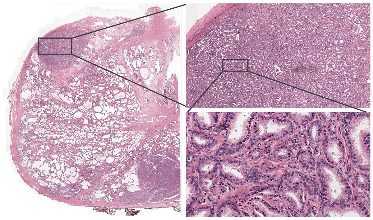
Besides H&E, other staining methods can highlight features of the tissue that are otherwise hidden or difficult to assess using H&E alone. Immunohistochemical (IHC) staining allows detecting specific proteins expressed by the cells contained in the tissue section. Although immunostaining highlights specific tissue proteins, assessing the overall architectural patterns of the tissue is difficult compared to H&E stained slides. Immunohistochemistry is also typically more expensive and resource-intensive as compared to the regular H&E staining. For prostate cancer, the tissue samples are typically assessed using H&E, while specific stains are used when additional evidence for a diagnosis is required.
Gleason grading system
Pathologists assess H&E stained prostate specimens following the Gleason grading system, which is the most important tissue-based prognostic marker for prostate cancer patients. Pathologists assess the architectural growth patterns of the tumor and assign it a number between 1 and 5, with increasing numbers corresponding to a decrease in histological differentiation and, typically, worse prognosis (Figure 1.5).18 While immunohistochemistry can be used to determine whether a case contains cancer, there is no specific stain that highlights Gleason patterns. Due to updates in the grading system, patterns 1 and 2 are not or rarely reported anymore for biopsies.1819 The detected patterns are then summarized in the Gleason score of a specimen.
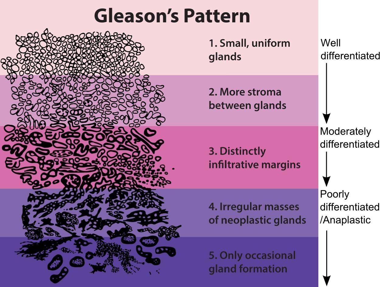
Overview of Gleason’s patterns. Due to changes in the grading system, patterns 1 and 2 are rarely reported anymore. Image: National Institutes of Health (SEER), public domain, via Wikimedia Commons.
For biopsies, the Gleason score is the sum of the most occurring pattern and the highest of the remaining patterns (e.g., 3+4=7). The second pattern should account for at least 5% of the tissue or be of a higher grade for it to be included in the reported score. For example, a biopsy with a majority pattern 4 and a second pattern 3 with a prevalence of 3% is assigned a score of 4+4=8. For the Gleason score of prostatectomies, the sum of the most common and the second most common pattern is used instead. Theoretically, the lowest Gleason score is 1+1=2, but in clinical practice the lowest reported Gleason score for a patient can be 3+3=6 and the highest 5+5=10.
Even though the grading system is clearly defined, prostate cancer is a heterogeneous disease with a wide range of tissue patterns, which complicates grading. The assessment of the tumor grade is a subjective and challenging process and therefore suffers from significant inter- and intraobserver variability.2021
A 5-tier grading system was introduced to improve the reporting of Gleason grading, which directly assigns Gleason scores to one of five prognostic groups (Figure 1.6).192223 Throughout the literature, the new grading system is referred to using different names, including (ISUP) grade group, Gleason grade groups, and ISUP grade. In this thesis, we use the general term grade group to refer to the new grading system. The groups, with the descriptions derived from Epstein et al.,19 are defined as follows:
- Grade Group 1: Gleason score 3+3=6, Only individual discrete well-formed glands.
- Grade group 2: Gleason score 3+4=7, Predominantly well-formed glands with lesser component of poorly-formed or fused or cribriform glands.
- Grade group 3: Gleason score 4+3=7, Predominantly poorly-formed, fused or cribriform glands with lesser component of well-formed glands.
- Grade group 4: Gleason scores 4+4=8, 3+5=8, 5+3=8, Either (1) only poorly-formed/fused/cribriform glands; (2) predominantly well-formed glands and lesser component lacking glands; or (3) predominantly lacking glands and a lesser component of well-formed glands.
- Grade group 5: Gleason scores 4+5=9, 5+4=9, 5+5=10, Lacks gland formation (or with necrosis) with or without poorly formed, fused, or cribriform glands.
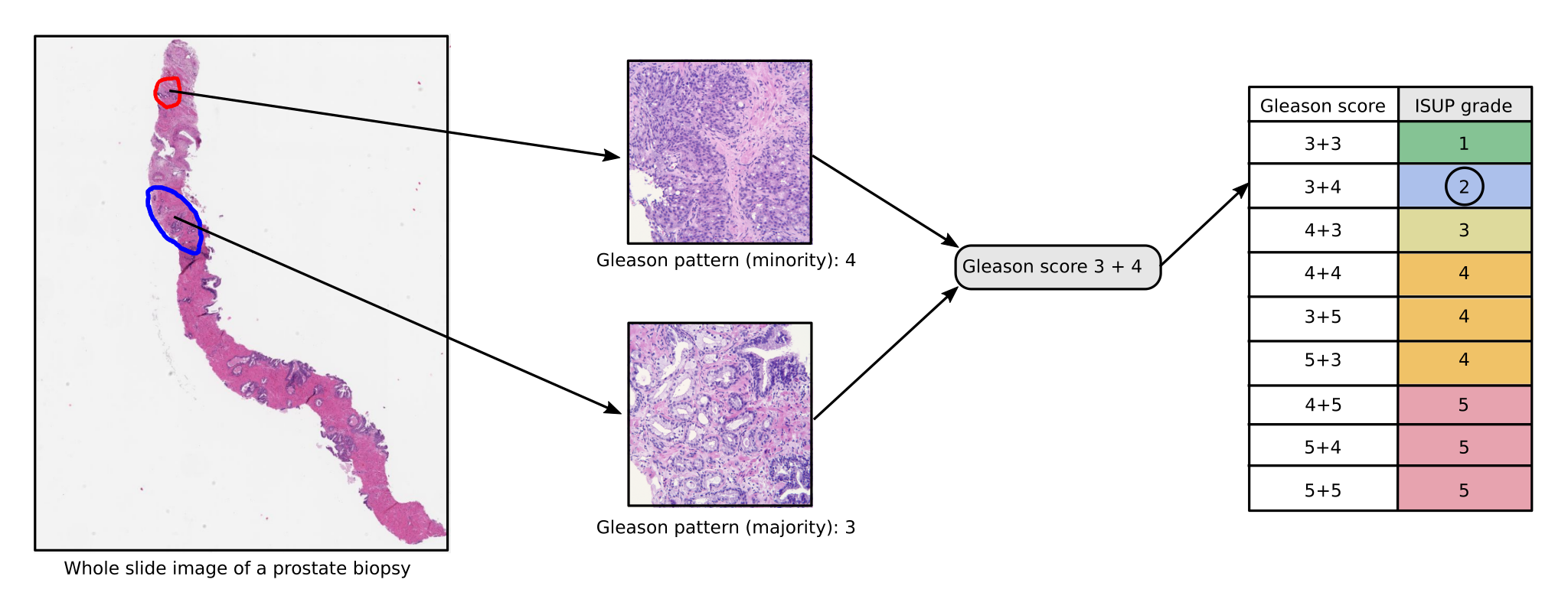
Grading system. Illustration by Kimmo Kartasalo.
The introduction of grade groups had two clear advantages. First, before the new system, the lowest reported score was a Gleason score 3+3=6, and a score of 6 out of 10 does not communicate the relatively positive prognosis well, especially to patients. Secondly, as there is a clear prognostic difference between Gleason score 3+4=7 and 4+3=7, the new grade group system explicitly communicates this by assigning these scores to different grade groups. While grade groups’ introduction showed clinical value and increased interpretability of the tumor grade for patients,24 there is also criticism on the simplification25, and it has not addressed the inter- and intraobserver variability.2627
Unfortunately, a small deviation in tumor grade can already have considerable implications for individual patients. For example, whereas the recommended treatment for grade group 1 is active surveillance, a change to group 2 could result in advice for radical therapy (e.g., surgery, radiotherapy).28 Whether a patient would receive surgery can depend on which pathologist handles their case. Research from The Netherlands showed that, when biopsies of patients were re-evaluated, 21% of cases were assigned a different grade, and in 43% of those cases, the original diagnosis was upgraded.29 Such re-evaluation is not common because of associated high costs and is only done in 3% of the cases, often when patients are referred to another hospital.
Specialized uropathologists show higher concordance rates in Gleason grading, but such expertise is not always available.30 This is furthermore complicated by a global shortage of pathologists we are increasingly witnessing,31 limiting access to accurate diagnostics for many patients. In Western countries, such as the UK and the USA, there is at least one pathologist per 50.000 patients, though the workload is high, and shortages are expected in the near future. This is in high contrast to, e.g., China with around 1 per 130.000 and Sub-Saharan Africa 1 per 1.000.000. These shortages are not expected to be solved soon, and a shortage or increase in workload is expected in western countries due to an aging population.
Digital & computational pathology
While the traditional pathologists’ workspace was, until recently, based on a microscope, this is slowly transitioning to diagnosis using a computer screen: Digital Pathology. This digital transition is made possible by the introduction of whole-slide scanners that are able to scan individual glass slides at high resolution, resulting in whole-slide images (WSI).
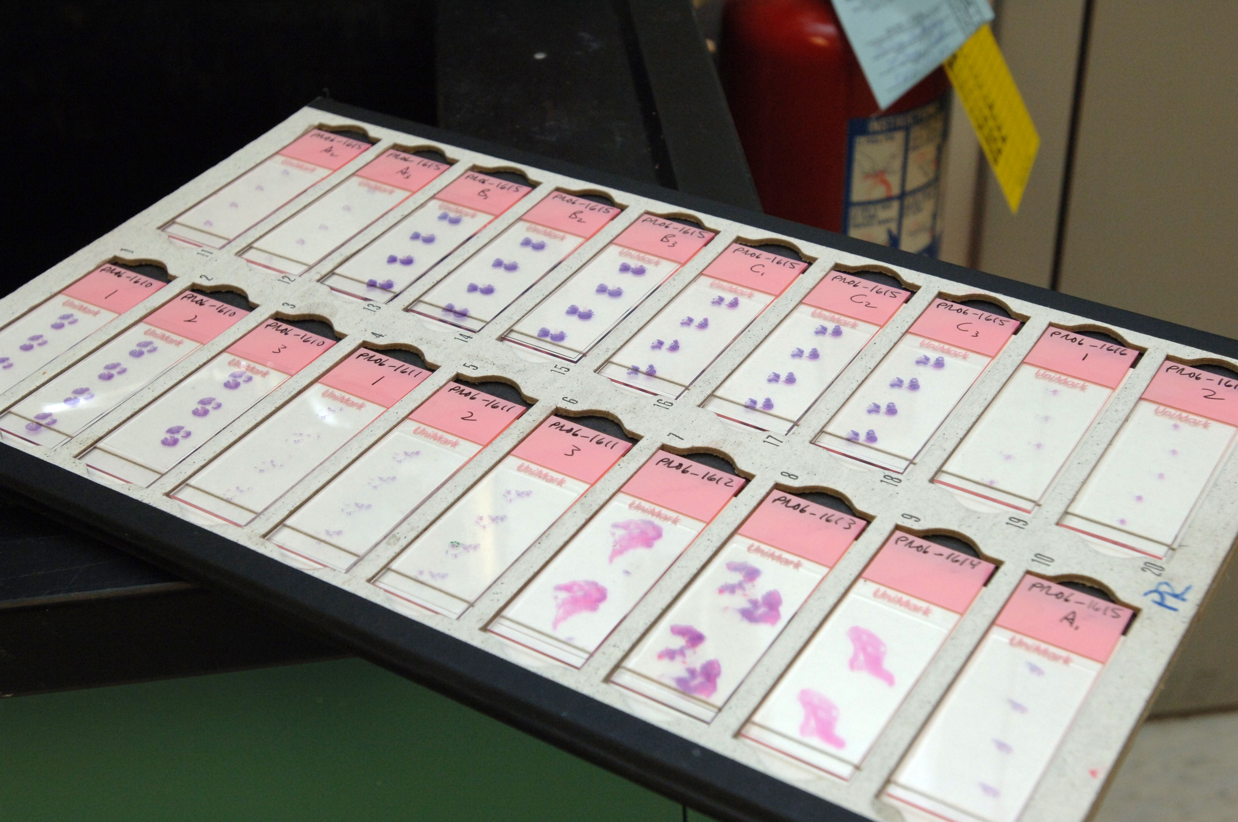
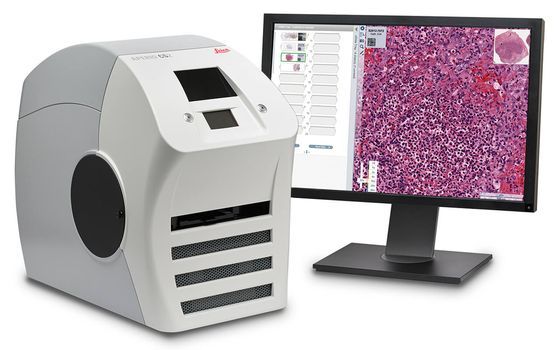
Glass slides with tissue sections (left) can be digitized using a whole-slide scanner (right). Slide tray photo by Ed Uthman via Wikimedia Commons; scanner photo: Leica Biosystems.
Histological assessment of tissue requires a pathologist to view the tissue at high magnification. To allow for digital assessment, a scanner takes a gigapixel image of the tissue, typically scanned at a resolution of 0.25-0.50 µm per pixel, corresponding to respectively a 40x and 20x objective of a traditional microscope. The pixel spacing of a scanned slide is crucial metadata as it defines how much area an individual pixel represents of the original tissue. A typical WSI can easily run up to 200.000 by 100.000 pixels, roughly corresponding to the same area as 1600 photos taken with a 12-megapixel camera. This considerable size introduces significant challenges in storing and management of these images.
WSIs are typically examined using specialized viewer software, which allows pathologists to efficiently navigate the image, zoom in on specific regions, and add annotations. One of those applications is the open-source ASAP viewer32 built on top of OpenSlide,33 which has been used as the main viewer during the conduct of the research in this thesis.
Digital pathology can have significant improvements on the histopathology workflow. Benefits of digital pathology include remote diagnostics, streamlined external consultation, and the ease of access to archived cases.34 Where traditionally fragile glass slides had to be shipped physically, digital pathology moves this transfer to the digital domain. Of course, this digital transition co-exists with significant digital infrastructure requirements and additional measures for privacy and data integrity.
The digital transition within pathology also allowed for a new research field to emerge: computational pathology.35 With histological slides now digitized, it is possible to annotate patterns in the tissue specimens digitally. This annotated data can then be used to develop computer models to assist in diagnosis.
Computer-aided diagnosis
The digitalization of various medical domains, including pathology, introduced the possibility of assisting medical professionals with (intelligent) algorithms that assist in or automate part of the diagnostic process. On an abstract level, these algorithms take patient data as input and transform this data into some outcome, potentially relevant to the task. Formalized, we can define such algorithms as a mapping from some input x to an output y:
This mapping can be simple, e.g., an algorithm that automatically computes the body-mass index (BMI) of a patient, which takes body weight and length as input:
While this example might sound trivial and would not be classified as an intelligent decision support tool, it highlights these algorithms’ basic structure. The same input-output-mapping definition holds for more complex systems, though these will have more elaborate inputs and outputs. The mapping function f() can be pre-defined, as in the BMI example, or learned. This thesis focuses on algorithms that take medical images as input and make predictions based on those images.
The assistance by algorithms can be performed on multiple abstraction levels, based on the output of the algorithm (Figure 1.8). At the lowest level, an algorithm could assist in the detection or quantification of certain structures. These are often referred to as computer-aided detection (CADe) or computer-aided quantification (CADq) systems. The task of such systems is to detect certain structures of interest in a medical image. Examples are the detection of lung nodules in CT,36 the detection of lymph node metastases,37 or the detection of prostate cancer in biopsies.38 Often, this detection is performed at a local level, so the input to the algorithm can also be limited, e.g., an algorithm could only require a small region around a lung nodule to detect it.
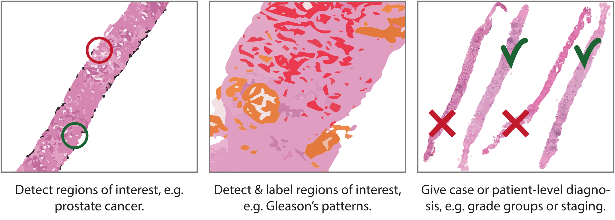
One level further concerns algorithms that focus on diagnosis, i.e., computer-aided diagnosis (CADx). These systems often are classification systems. Besides detecting specific objects of interest, these algorithms also need to classify the detected objects into pre-defined groups or classes. Examples of such classification systems are the classification of lymph node metastases in either micro, macro, or isolated tumor cells,39 or the assignment of Gleason patterns to individual prostate glands. Depending on the task, such systems could require a more extensive input. E.g., for detecting Gleason patterns, the surrounding area of a gland is required to make an accurate assessment of the morphology.
On the highest abstraction level, systems give feedback or output on a case or patient level. Algorithms that perform this task, especially in medical imaging, are often more complicated, as such systems take low-level input and transform this to high-level predictions. An example for prostate cancer could be the biopsy-level diagnosis, which summarizes the detected tissue patterns in a single grade group. On a patient-level, usually, information from multiple images is combined, e.g., the staging of a set of lymph nodes39 or the prognosis for an individual patient.
The names for the different abstraction levels of intelligent algorithms are often used interchangeably. In this thesis, we will use the general term computer-aided diagnosis (CAD), deep learning system, or algorithm as an overarching term.
Deep learning
Traditionally, CAD systems for medical imaging were designed by hand with so-called “hand-crafted features.” Based on domain knowledge, researchers would engineer quantitative features to extract information from an image and create a representation on which machine learning models could be trained. Such algorithms can be seen as a two-step approach. First, the input is transformed using some pre-defined feature extractor function h(), after which a machine learning model f() is trained to map these features to the desired output y:
This two-step approach was mostly due to machine learning techniques’ inability to learn from the raw data directly. Though, a minor benefit of this approach is that it is an easy way to introduce expert knowledge into the algorithm. However, this comes at the cost of having to pre-define the features instead of learning these directly from the data itself.
Currently, the field has almost entirely transitioned to using feature or representation learning. Instead of hand-crafting the features, the features are learned automatically from the raw data. At the basis is a technique that has been around for years: artificial neural networks.40 Such networks consist of connected artificial neurons (Figure 1.9), which through connections between the neurons form a network. Each neuron is a simple mapping function, but these networks can model complex functions as a whole. When there are many layers of neurons in a network, we speak of a deep neural network and the more general term: deep learning.
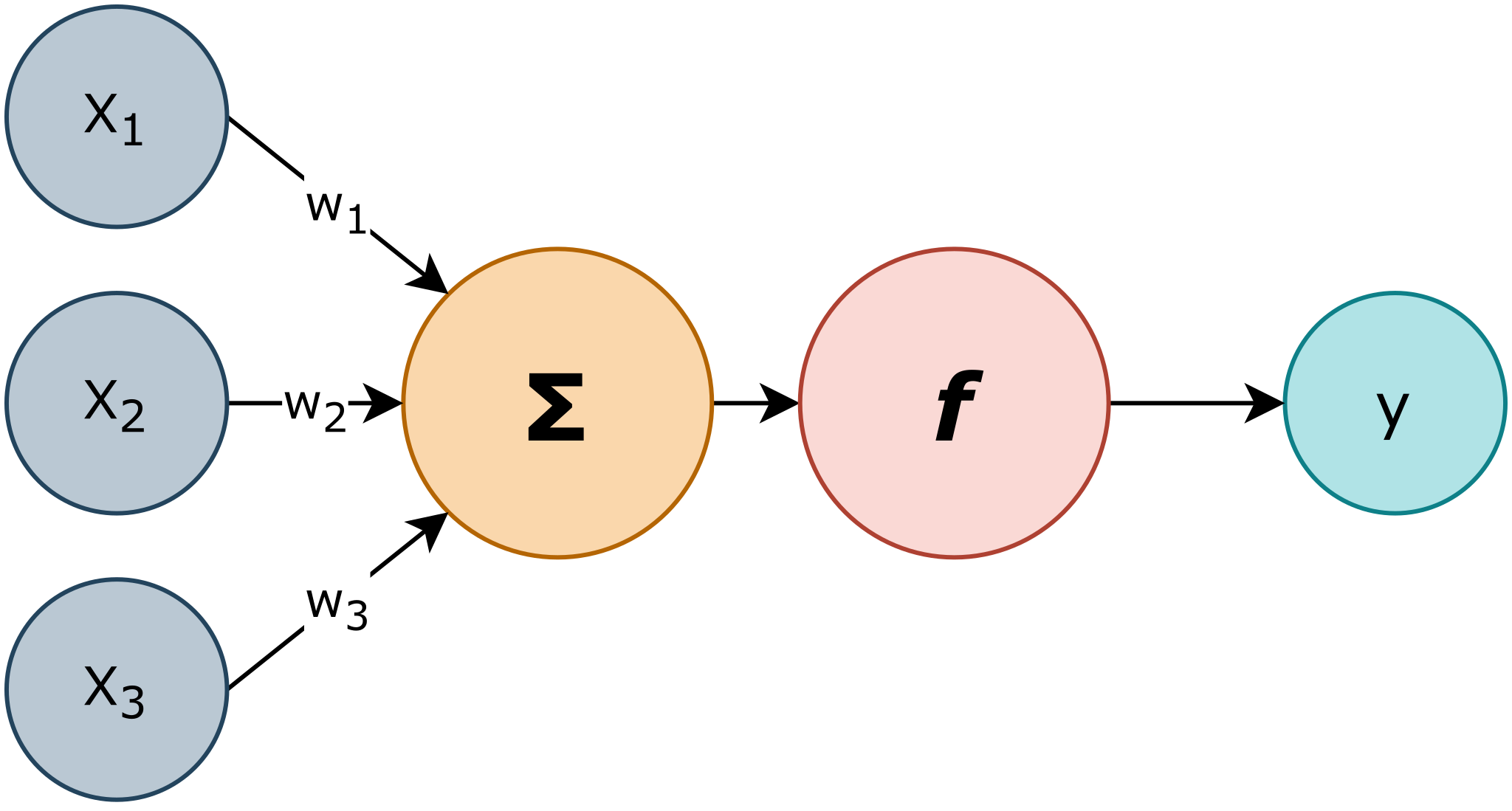
Historically, artificial neural networks, specifically multilayer perceptrons,41 consisted of fully connected layers in which each neuron was connected to all neurons in the previous layer. This architecture made those networks prone to overfitting and deep networks infeasible due to the memory requirements.
In recent years, advances have been made in the training of deep neural networks, further boosted due to the developments in hardware technology, specifically fast graphics processing units (GPUs). Due to these developments, the field underwent a deep learning revolution,4243 making deep learning-based approaches the de-facto standard for many image analysis tasks. A famous example is a study by Krizhevsky et al. on the ImageNet classification task, whose deep learning approach outperformed the previous non-deep learning approaches by a wide margin.44 The availability of many high-quality Open Source tools for deep learning has also stimulated further development.4549
One specific subtype of neural networks is crucial for computer vision: convolutional neural networks (CNN). Instead of the fully connected networks, CNNs instead use small filters that are slided over the input image at each valid position to compute the output. The benefit of these filters is that they are invariant to translations, as each filter is applied to every possible valid input region of the image. This approach makes CNNs highly effective for image analysis. Deeper into the network, each layer will respond to more complex features in the images, which is why CNNs and filters are often compared to the visual cortex (Figure 1.10).4350
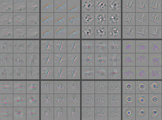
Layers in convolutional neural networks are often compared to the visual cortex. Early layers (left) respond to simple features, while deeper layers (right) react to more complex input patterns. Images adapted from Zeiler et al.51
A CNN consists of multiple building blocks that stacked together form the final network. Layers are connected in the form of a directed acyclic graph, where each layer represents a node to form the CNN. In its basic form, each layer directly follows the previous layer. More complex architectures use, e.g., skip connections or concatenation operations to introduce additional parallel paths inside the network.
While many variants and subvariants of these building blocks exist, there are a few of these that are often used:
- Convolutional layers are at the core of a CNN and apply the filters to the input image. The number of filters per layer can differ and is often increased for deeper layers. Filters in earlier layers often react to basic features, while deeper layers typically respond to more complex structures of the input domain (Figure 1.10).51
- Activation layers apply a function to their input. From the biological perspective, this layer determines whether a neuron fires. These functions are often nonlinear.
- Pooling layers perform a summary function, e.g., average or maximum, on a window of the input. Pooling layers downsample the input, resulting in a smaller input for subsequent layers and a larger field of view. Upsampling layers can reverse pooling layers, which is a key element of the popular U-Net architecture.52
- Fully connected layers are often used in the last part of a network to perform the final classification. At this point in the network, the previous layers have already extracted relevant features from the data, and the role of the fully connected layers is to incorporate this information in a final prediction. A convolutional layer can also emulate a fully connected layer by using a kernel size of 1. Doing this creates a fully convolutional neural network that can easily scale to larger input sizes.53
Challenges for computational pathology
The field of computational pathology is characterized by specific challenges that distinguish it from other (medical) imaging domains. Here we discuss the three challenges most relevant to this thesis: the gigapixel size of the slides, artifacts, and variations in the images caused by different scanners and labs.
The first challenge is the size of the whole-slide images. Glass slides are typically scanned at 40× or 20× magnification, resulting in gigapixel-sized images with dimensions of 200.000×100.000 pixels being no exception. Because of this size, exhaustively annotating all the tissue by hand is often infeasible or cost-ineffective for large datasets. Technically, annotating these slides by hand is still possible, but limited resources require innovative approaches to acquire enough training data.
Besides an enormous annotation burden, the image’s size introduces technical problems during the training of neural networks. These gigapixel images do not fit a modern GPU’s memory at full resolution, limiting options for training deep learning models on the full image. While it is possible to downscale the whole-slide image to a resolution that would fit the GPU, this removes the necessary detail for many diagnostic tasks.
Instead of using the entire image, deep learning systems for pathology are typically trained in a so-called “patch-based” manner (Figure 1.11). The full image is split into small tiles (patches) that do fit into GPU memory and are then used for training. The same approach is utilized when a deep learning system needs to classify an unseen case (i.e., inference). The final prediction can be formed by processing the case tile-by-tile and stitching the output together.
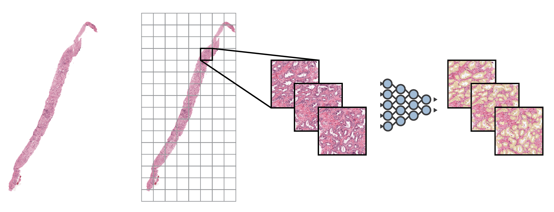
In its typical form, patch-based training requires that individual patches are independent of each other, as the field of view of the deep learning system is limited to a single patch’s dimensions. For many tasks, this is not a limitation as predictions can be made using a relatively small field of view. However, if more global information is required, e.g., structure’s position within the tissue, solely relying on patch-based training will not work. A second limitation of patch-based training is that each patch requires a label. Due to large images in pathology, a slide-level label is not always represented by each patch. For example, a biopsy containing a tumor could have a slide-level label of ‘malignant,’ but not every region in that biopsy has to contain cancer.
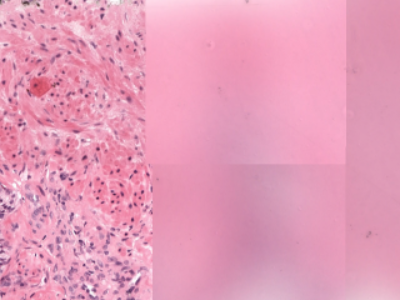
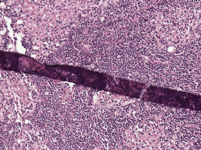
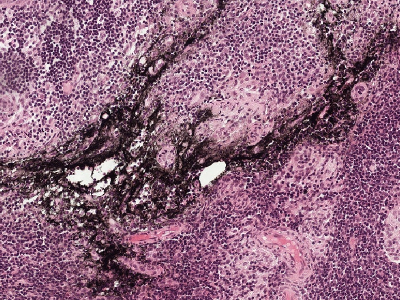
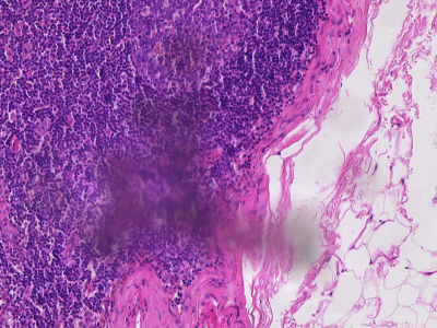
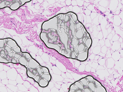
A second challenge for automated analysis of histological slides is the presence of artifacts (Figure 1.12). The road from patient to a digitized slide of a patient’s tissue sample is long, and in each step of the process, artifacts can be introduced.54 An overview of common artifacts:
- Out-of-focus regions are caused by incorrect focus points of digital pathology scanners. Typically scanners start with a low-resolution scan to determine focus points. If these focus points are set incorrectly, parts of the tissue will be rendered out-of-focus, which hinders the tissue’s assessment (Figure 1.12a).
- Tissue folds occur during handling of the tissue sections. A fold distorts the tissue and can be recognized by a typical darker well-demarcated line (Figure 1.12b). Sometimes a tissue fold also introduces blurring artifacts if the scanner selected an incorrect focus point due to the tissue fold being thicker than the surrounding area.
- Ink is often used to aid the identification of tissue samples. For example, biopsies can be inked with distinct colors before cutting and then placed on the same glass slide. The presence of ink helps to identify the biopsies in the final scan. Unfortunately, (excessive use of) ink can also obscure some of the tissue and result in misclassifications by deep learning systems (Figure 1.12c).
- Dust, air bubbles or even eyelashes of the technician can end up under the coverslip. After scanning, these artifacts will be clearly visible in the image (Figure 1.12d and 1.12e).
- Pen markings are commonly present in archived glass slides. In the era of the microscope, pen markings were an easy way of annotating or outlining tissue regions for future reference. When scanning large sets of archived slides, it can be expected that these pen markings are present if the slides are not cleaned first (Figure 1.12f). Due to the introduction of digital pathology, the presence of pen markings will decrease over time.
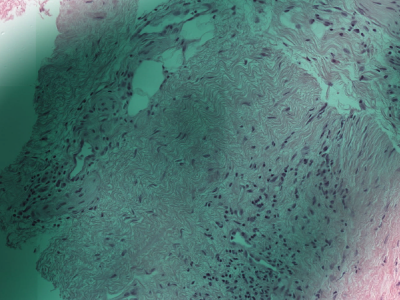
The last challenge regards scanner and stain variations. Image characteristics can vary wildly based on the lab that stained the tissue and the scanner that digitized the glass slide (Figure 1.13).56 These variations can be challenging for deep learning methods if the algorithm is purely trained on data from a single center and needs to be applied to data from a different center.

Examples of breast tissue samples stained with H&E from different centers.55 Even though the same stain is used, because the tissue is stained in different centers, there is significant stain variance. Examples from Veta et al., 2019.
Some of the variations can be circumvented through simple measures. For example, discrepancies in the pixel spacing between scanners can often be reduced by resizing the image, e.g., when an image is scanned at a pixel resolution of 0.26µm, and the network was trained on data scanned with a resolution of 0.24µm. Stain normalization or transformation techniques can also be used to reduce stain variations.5761
Alternatively, algorithms can be trained using data augmentation that tries to simulate stain variations and scanner characteristics.62 In this approach, instead of trying to remove variation in the new data, additional variation is introduced during the training phase.
Aims and objectives
The histological grading of prostate biopsies is a crucial element in the diagnostic pathway of prostate cancer. The known high inter- and intraobserver variability show potential and a need for assisting pathologists in this task. Furthermore, a global shortage of pathologists stresses the demand for reproducible, more efficient, and easily accessible diagnostic solutions.
This thesis’s primary aim was to investigate and design an AI-based system to detect and grade prostate cancer in biopsies. A second aim was to evaluate the potential clinical merits of AI-assisted grading when such systems are embedded in the pathologist’s workflow. To this extent, the following objectives were undertaken as part of this thesis:
- The development of an automated system that can distinguish epithelial tissue from other tissue types within H&E stained prostate specimens (Chapter 2);
- The development and validation of an automated system for grading prostate biopsies using the Gleason grading system (Chapter 3);
- A multi-center independent evaluation of state-of-the-art algorithms for automated Gleason grading sourced through a large-scale medical AI competition (Chapter 4);
- The investigation of the potential merits of AI-assisted grading of prostate cancer through an observer study (Chapter 5).
Thesis outline
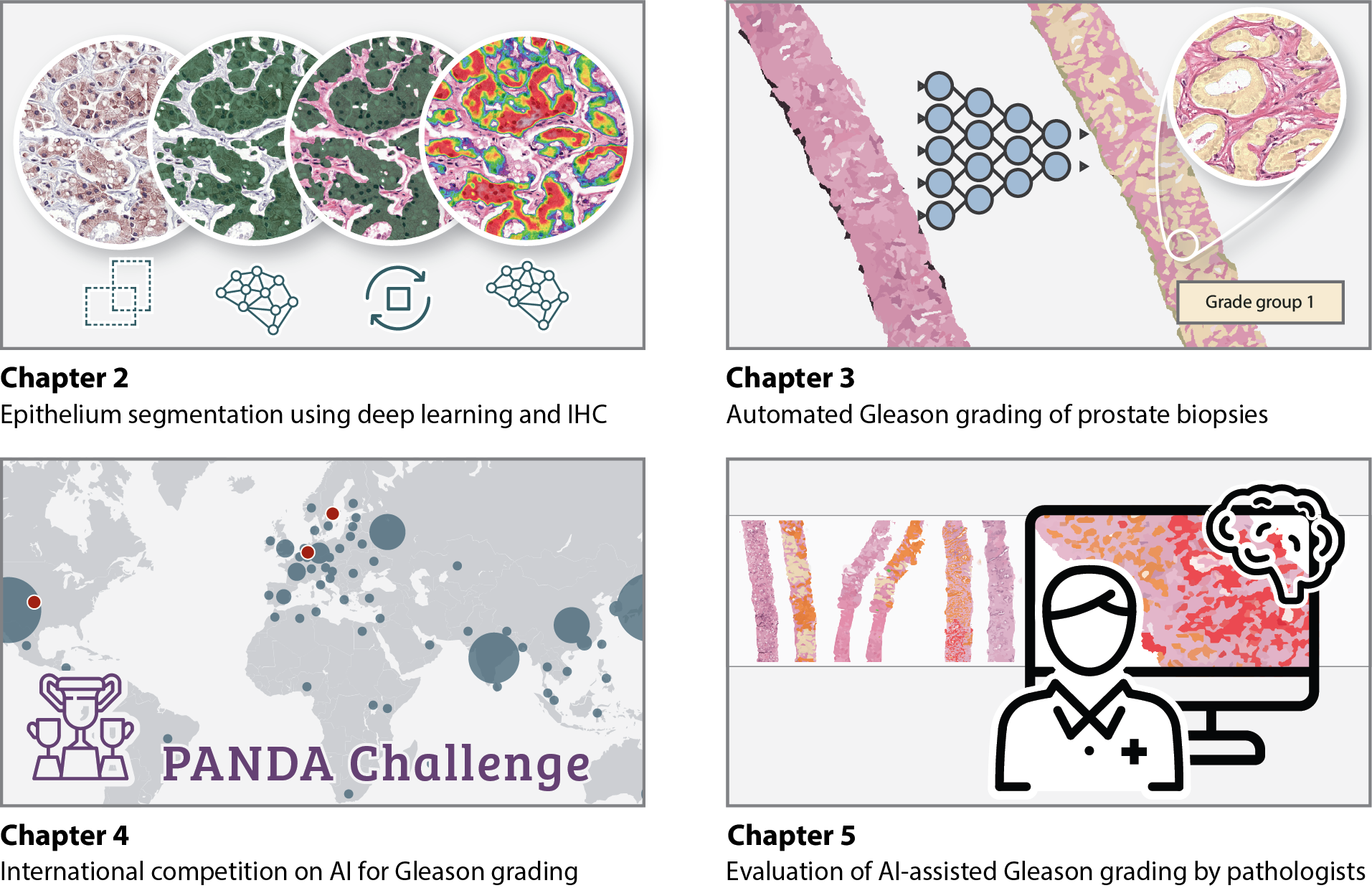
The remainder of this thesis is organized in the following chapters (Figure 1.14):
- Chapter 2 Detecting epithelial tissue in H&E can be seen as a prerequisite for the detection and grading of prostate cancer. Manual annotation of epithelial tissue is complicated by the heterogeneous character of epithelial tissue within the prostate, ranging from intact glands to strands of individual cells. This chapter describes a method to train a deep learning system to segment epithelial tissue using immunohistochemistry as the reference standard, alleviating the need for manual annotations.
- Chapter 3 In order to assist pathologists when grading prostate cancer, deep learning methods need to achieve pathologist-level performance. This chapter investigates the development and validation of a deep learning system for the diagnosis of prostate cancer in biopsies. For the development of the deep learning system, a completely new cohort of prostate cancer patients was collected. Furthermore, the deep learning system is compared to pathologists on several clinically relevant decision thresholds.
- Chapter 4 Clinical implementations of automated Gleason grading requires algorithms that perform well in a multi-center setting. In this chapter, several state-of-the-art algorithms are investigated and independently validated using data from multiple centers through an international competition: the PANDA challenge.
- Chapter 5 When AI algorithms have shown to achieve pathologist-level performance at diagnosing prostate cancer, it remains to be investigated how this could benefit clinical diagnostics. This chapter investigates the effect of AI assistance on Gleason grading by pathologists.
- Chapter 6 The final chapter summarizes the key contributions of this research and discusses the implications and future work.
References
- Bray F, Ferlay J, Soerjomataram I, Siegel RL, Torre LA, Jemal A. Global cancer statistics 2018: GLOBOCAN estimates of incidence and mortality worldwide for 36 cancers in 185 countries. CA: A Cancer Journal for Clinicians. 2018;68(6):394–424. doi:10.3322/caac.21492
- Crawford ED. Epidemiology of prostate cancer. Urology. 2003;62(6, Supplement 1):3–12. doi:10.1016/j.urology.2003.10.013
- Ferlay J, Ervik M, Lam F, Colombet M, Mery L, Piñeros M, et al. Global Cancer Observatory: Cancer Tomorrow. Accessed November 7, 2020. https://gco.iarc.fr/tomorrow
- IKNL. Nederlandse Kankerregistratie (NKR). Accessed July 14, 2020. http://iknl.nl/nkr-cijfers
- Schröder FH, Hugosson J, Roobol MJ, Tammela TLJ, Ciatto S, Nelen V, et al. Prostate-cancer mortality at 11 years of follow-up. New England Journal of Medicine. 2012;366:981–990. doi:10.1056/NEJMoa1113135
- McNeal JE, Redwine EA, Freiha FS, Stamey TA. Zonal distribution of prostatic adenocarcinoma: correlation with histologic pattern and direction of spread. The American journal of surgical pathology. 1988;12(12):897–906.
- Lee JJ, Thomas IC, Nolley R, Ferrari M, Brooks JD, Leppert JT. Biologic differences between peripheral and transition zone prostate cancer. The Prostate. 2015;75(2):183–190.
- Augustin H, Erbersdobler A, Graefen M, Fernandez S, Palisaar J, Huland H, et al. Biochemical recurrence following radical prostatectomy: a comparison between prostate cancers located in different anatomical zones. The Prostate. 2003;55(1):48–54.
- Schröder FH, Hugosson J, Roobol MJ, Tammela TLJ, Ciatto S, Nelen V, et al. Screening and Prostate-Cancer Mortality in a Randomized European Study. New England Journal of Medicine. 2009;360(13):1320–1328. doi:10.1056/NEJMoa0810084
- Hugosson J, Roobol MJ, Månsson M, Tammela TLJ, Zappa M, Nelen V, et al. A 16-yr Follow-up of the European Randomized study of Screening for Prostate Cancer. European Urology. 2019;76(1):43–51. doi:10.1016/j.eururo.2019.02.009
- Heijnsdijk EAM, Wever EM, Auvinen A, Hugosson J, Ciatto S, Nelen V, et al. Quality-of-Life Effects of Prostate-Specific Antigen Screening. New England Journal of Medicine. 2012;367(7):595–605. doi:10.1056/nejmoa1201637
- Federatie van Medisch Specialisten. Prostaatcarcinoom Richtlijn - Korte beschrijving. Accessed July 22, 2020. https://richtlijnendatabase.nl/richtlijn/prostaatcarcinoom/prostaatcarcinoom_-_korte_beschrijving.html
- Nederlands Huisartsen Genootschap. Mictieklachten bij mannen. Accessed July 22, 2020. https://richtlijnen.nhg.org/standaarden/mictieklachten-bij-mannen
- Federatie van Medisch Specialisten. Prostaatcarcinoom Richtlijn - Prostaatbiopten. Accessed July 22, 2020. https://richtlijnendatabase.nl/richtlijn/prostaatcarcinoom/pathologisch_onderzoek/prostaatbiopten.html
- Eichler K, Hempel S, Wilby J, Myers L, Bachmann LM, Kleijnen J. Diagnostic value of systematic biopsy methods in the investigation of prostate cancer: a systematic review. The Journal of urology. 2006;175(5):1605–1612.
- Bladou F, Fogaing C, Levental M, Aronson S, Alameldin M, Anidjar M. Transrectal ultrasound-guided biopsy for prostate cancer detection: Systematic and/or magnetic-resonance imaging-targeted. Canadian Urological Association Journal. 2017;11(9):E330.
- Federatie van Medisch Specialisten. Prostaatcarcinoom Richtlijn - Diagnostische prostaat MRI. Accessed July 22, 2020. https://richtlijnendatabase.nl/richtlijn/prostaatcarcinoom/diagnostiek/beeldvormend_onderzoek/diagnostische_prostaat_mri_bij_prostaatcarcinoom.html
- Epstein JI, Allsbrook WC, Amin MB, Egevad LL, Bastacky S, López Beltrán A, et al. The 2005 International Society of Urological Pathology (ISUP) consensus conference on Gleason grading of prostatic carcinoma. American Journal of Surgical Pathology. 2005;29(9):1228–1242. doi:10.1097/01.pas.0000173646.99337.b1
- Epstein JI, Egevad L, Amin MB, Delahunt B, Srigley JR, Humphrey PA. The 2014 International Society of Urological Pathology (ISUP) Consensus Conference on Gleason Grading of Prostatic Carcinoma. The American Journal of Surgical Pathology. 2016;40(2):1. doi:10.1097/pas.0000000000000530
- Allsbrook WC, Mangold KA, Johnson MH, Lane RB, Lane CG, Epstein JI. Interobserver reproducibility of Gleason grading of prostatic carcinoma: General pathologists. Human Pathology. 2001;32(1):81–88. doi:10.1053/hupa.2001.21135
- Egevad L, Ahmad AS, Algaba F, Berney DM, Boccon-Gibod L, Compérat E, et al. Standardization of Gleason grading among 337 European pathologists. Histopathology. 2013;62(2):247–256. doi:10.1111/his.12008
- Epstein JI, Zelefsky MJ, Sjoberg DD, Nelson JB, Egevad L, Magi-Galluzzi C, et al. A Contemporary Prostate Cancer Grading System: A Validated Alternative to the Gleason Score. European urology. 2016;69(3):428–435. doi:10.1016/j.eururo.2015.06.046
- Van Leenders GJ, Van Der Kwast TH, Grignon DJ, Evans AJ, Kristiansen G, Kweldam CF, et al. The 2019 International Society of Urological Pathology (ISUP) consensus conference on grading of prostatic carcinoma. The American journal of surgical pathology. 2020;44(8):e87.
- Loeb S, Folkvaljon Y, Robinson D, Lissbrant IF, Egevad L, Stattin P. Evaluation of the 2015 Gleason grade groups in a nationwide population-based cohort. European urology. 2016;69(6):1135–1141.
- Egevad L, Delahunt B, Bostwick DG, Cheng L, Evans AJ, Gianduzzo T, et al. Prostate cancer grading, time to go back to the future. BJU international. 2020.
- Ozkan TA, Eruyar AT, Cebeci OO, Memik O, Ozcan L, Kuskonmaz I. Interobserver variability in Gleason histological grading of prostate cancer. Scandinavian Journal of Urology. 2016;50(6):420–424. doi:10.1080/21681805.2016.1206619
- Nagpal K, Foote D, Liu Y, Chen PHC, Wulczyn E, Tan F, et al. Development and validation of a deep learning algorithm for improving Gleason scoring of prostate cancer. npj Digital Medicine. 2019;2(1):48. doi:10.1038/s41746-019-0112-2
- Federatie van Medisch Specialisten. Prostaatcarcinoom Richtlijn - Behandeling gelokaliseerd prostaatcarcinoom. Accessed February 8, 2021. https://richtlijnendatabase.nl/richtlijn/prostaatcarcinoom/gelokaliseerd_prostaatcarcinoom.html
- van Santvoort BWH, van Leenders GJLH, Kiemeney LA, van Oort IM, Wieringa SE, Jansen H, et al. Histopathological re-evaluations of biopsies in prostate cancer: a nationwide observational study. Scandinavian Journal of Urology. 2020;0(0):1–7. doi:10.1080/21681805.2020.1806354
- Allsbrook WC, Mangold KA, Johnson MH, Lane RB, Lane CG, Amin MB, et al. Interobserver reproducibility of Gleason grading of prostatic carcinoma: Urologic pathologists. Human Pathology. 2001;32(1):74–80. doi:10.1053/hupa.2001.21134
- Wilson ML, Fleming KA, Kuti MA, Looi LM, Lago N, Ru K. Access to pathology and laboratory medicine services: a crucial gap. The Lancet. 2018;391(10133):1927–1938.
- Litjens G. ASAP - Automated Slide Analysis Platform. 2015.
- Goode A, Gilbert B, Harkes J, Jukic D, Satyanarayanan M. OpenSlide: A vendor-neutral software foundation for digital pathology. Journal of pathology informatics. 2013;4.
- Griffin J, Treanor D. Digital pathology in clinical use: where are we now and what is holding us back? Histopathology. 2017;70(1):134–145.
- Abels E, Pantanowitz L, Aeffner F, Zarella MD, van der Laak J, Bui MM, et al. Computational pathology definitions, best practices, and recommendations for regulatory guidance: a white paper from the Digital Pathology Association. The Journal of pathology. 2019;249(3):286–294.
- Setio AAA, Traverso A, de Bel T, Berens MSN, Bogaard CVD, Cerello P, et al. Validation, comparison, and combination of algorithms for automatic detection of pulmonary nodules in computed tomography images: The LUNA16 challenge. Medical Image Analysis. 2017;42:1–13. doi:10.1016/j.media.2017.06.015
- Ehteshami Bejnordi B, Veta M, van Diest PJ, van Ginneken B, Karssemeijer N, Litjens G, et al. Diagnostic Assessment of Deep Learning Algorithms for Detection of Lymph Node Metastases in Women With Breast Cancer. Journal of the American Medical Association. 2017;318(22):2199–2210. doi:10.1001/jama.2017.14585
- Litjens G, Sánchez CI, Timofeeva N, Hermsen M, Nagtegaal I, Kovacs I, et al. Deep learning as a tool for increased accuracy and efficiency of histopathological diagnosis. Nature Scientific Reports. 2016;6:26286. doi:10.1038/srep26286
- Bándi P, Geessink O, Manson Q, van Dijk M, Balkenhol M, Hermsen M, et al. From detection of individual metastases to classification of lymph node status at the patient level: the CAMELYON17 challenge. IEEE Transactions on Medical Imaging. 2018;38(2):550–560. doi:10.1109/tmi.2018.2867350
- Russell S, Norvig P. Artificial intelligence: a modern approach. Prentice Hall. 2002.
- Rosenblatt F. The perceptron, a perceiving and recognizing automaton Project Para. Cornell Aeronautical Laboratory. 1957.
- Goodfellow I, Bengio Y, Courville A. Deep Learning. MIT Press. 2016. http://www.deeplearningbook.org
- LeCun Y, Bengio Y, Hinton G. Deep learning. Nature. 2015;521(7553):436–444.
- Krizhevsky A, Sutskever I, Hinton GE. Imagenet classification with deep convolutional neural networks. Advances in neural information processing systems. 2012;25:1097–1105.
- Theano Development Team. Theano: A Python framework for fast computation of mathematical expressions. arXiv e-prints. 2016;abs/1605.02688. http://arxiv.org/abs/1605.02688
- Dieleman S, Schlüter J, Raffel C, Olson E, Sønderby SK, Nouri D, et al. Lasagne: First release. 2015. doi:10.5281/zenodo.27878
- Abadi M, et al. TensorFlow: Large-Scale Machine Learning on Heterogeneous Systems. 2015. Software available from tensorflow.org. https://www.tensorflow.org/
- Chollet F, et al. Keras. GitHub. 2015. https://github.com/keras-team/keras
- Paszke A, Gross S, Massa F, Lerer A, Bradbury J, Chanan G, et al. PyTorch: An Imperative Style, High-Performance Deep Learning Library. In: Advances in Neural Information Processing Systems 32. Curran Associates, Inc; 2019:8024–8035. http://papers.neurips.cc/paper/9015-pytorch-an-imperative-style-high-performance-deep-learning-library.pdf
- Cadieu CF, Hong H, Yamins DL, Pinto N, Ardila D, Solomon EA, et al. Deep neural networks rival the representation of primate IT cortex for core visual object recognition. PLoS Computational Biology. 2014;10(12):e1003963.
- Zeiler MD, Fergus R. Visualizing and understanding convolutional networks. In: European conference on computer vision. Springer; 2014:818–833.
- Ronneberger O, Fischer P, Brox T. U-Net: Convolutional Networks for Biomedical Image Segmentation. In: Medical Image Computing and Computer-Assisted Intervention. Lecture Notes in Computer Science. Vol 9351. 2015:234–241.
- Shelhamer E, Long J, Darrell T. Fully Convolutional Networks for Semantic Segmentation. In: Proceedings of the IEEE Conference on Computer Vision and Pattern Recognition. 2015:3431–3440. doi:10.1109/TPAMI.2016.2572683
- Taqi SA, Sami SA, Sami LB, Zaki SA. A review of artifacts in histopathology. Journal of oral and maxillofacial pathology: JOMFP. 2018;22(2):279.
- Veta M, Heng YJ, Stathonikos N, Bejnordi BE, Beca F, Wollmann T, et al. Predicting breast tumor proliferation from whole-slide images: the TUPAC16 challenge. Medical image analysis. 2019;54:111–121.
- Clarke EL, Treanor D. Colour in digital pathology: a review. Histopathology. 2017;70(2):153–163.
- Bejnordi BE, Litjens G, Timofeeva N, Otte-Höller I, Homeyer A, Karssemeijer N, et al. Stain specific standardization of whole-slide histopathological images. IEEE transactions on medical imaging. 2015;35(2):404–415.
- Janowczyk A, Basavanhally A, Madabhushi A. Stain normalization using sparse autoencoders (StaNoSA): application to digital pathology. Computerized Medical Imaging and Graphics. 2017;57:50–61.
- Bug D, Schneider S, Grote A, Oswald E, Feuerhake F, Schüler J, et al. Context-based normalization of histological stains using deep convolutional features. In: Deep Learning in Medical Image Analysis and Multimodal Learning for Clinical Decision Support. Springer; 2017:135–142.
- Zanjani FG, Zinger S, Bejnordi BE, van der Laak JA, de With PH. Stain normalization of histopathology images using generative adversarial networks. In: 2018 IEEE 15th International Symposium on Biomedical Imaging (ISBI 2018). IEEE; 2018:573–577.
- de Bel T, Hermsen M, Kers J, van der Laak J, Litjens G. Stain-Transforming Cycle-Consistent Generative Adversarial Networks for Improved Segmentation of Renal Histopathology. In: Proceedings of The 2nd International Conference on Medical Imaging with Deep Learning. Proceedings of Machine Learning Research. Vol 102. PMLR; 2019:151–163. http://proceedings.mlr.press/v102/de-bel19a.html
- Tellez D, Litjens G, Bandi P, Bulten W, Bokhorst JM, Ciompi F, et al. Quantifying the effects of data augmentation and stain color normalization in convolutional neural networks for computational pathology. Medical Image Analysis. 2019;58:101544. doi:10.1016/j.media.2019.101544
Feedback? Questions?
Do you have a question or comment about this post? Feel free to reach out to me via the contact page.