Automated Gleason grading of prostate biopsies
This is chapter 3 of my PhD thesis, defended at Radboud University in . The text is adapted from the accepted manuscript of the paper below, not from the published version, and differs from it in wording and layout, but the data, results and conclusions are the same.
Want the short version? I wrote about this work on the blog:
- Adapted from
- Automated deep-learning system for Gleason grading of prostate cancer using biopsies: a diagnostic study
- Published in
- The Lancet Oncology 21(2), 233–241 (2020). doi:10.1016/S1470-2045(19)30739-9
- Authors
-
Wouter Bulten, Hans Pinckaers, Hester van Boven and 6 more Wouter Bulten, Hans Pinckaers, Hester van Boven, Robert Vink, Thomas de Bel, Bram van Ginneken, Jeroen van der Laak, Christina Hulsbergen-van de Kaa, Geert Litjens
- Licence
- this chapter is shared under CC BY-NC-ND 4.0. The published article is © 2020 Elsevier Ltd.
On this page 9 sections
- Abstract
- Introduction
- Methods
- Study design and participants
- Test methods
- Statistical analysis
- Role of the funding source
- Results
- Dataset & reference standard
- Performance on the internal test set
- Comparison to a panel of pathologists
- Performance on the external test set
- Discussion
- Acknowledgements
- Supplementary figures
- Grade group agreement (quadratic kappa) between panel and deep learning system
- Accuracy deep learning system accuracy versus panel
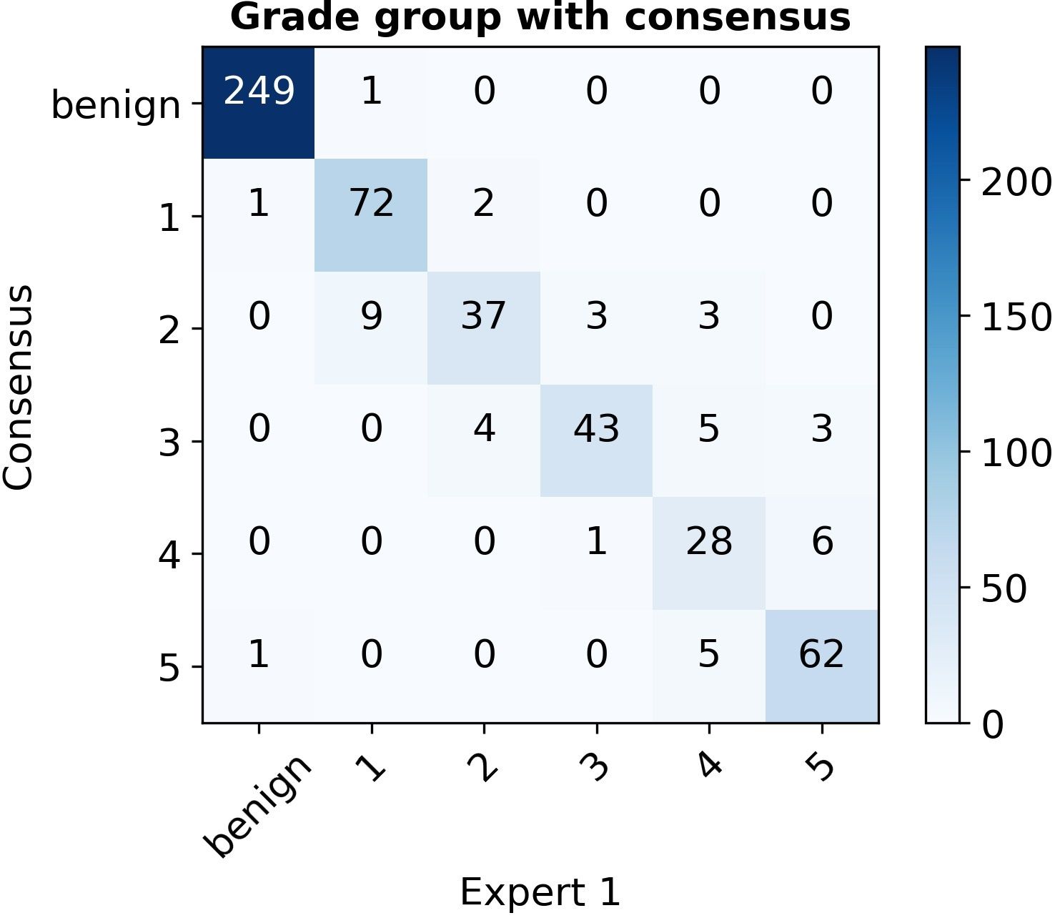
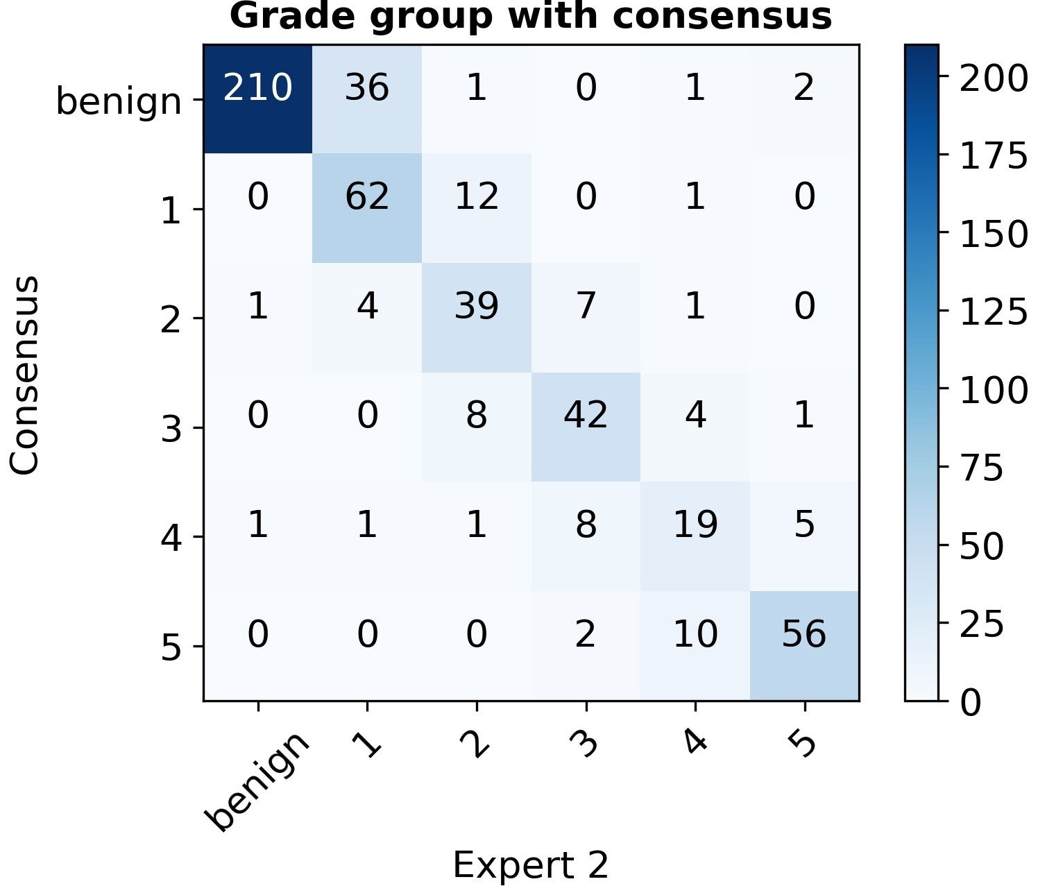
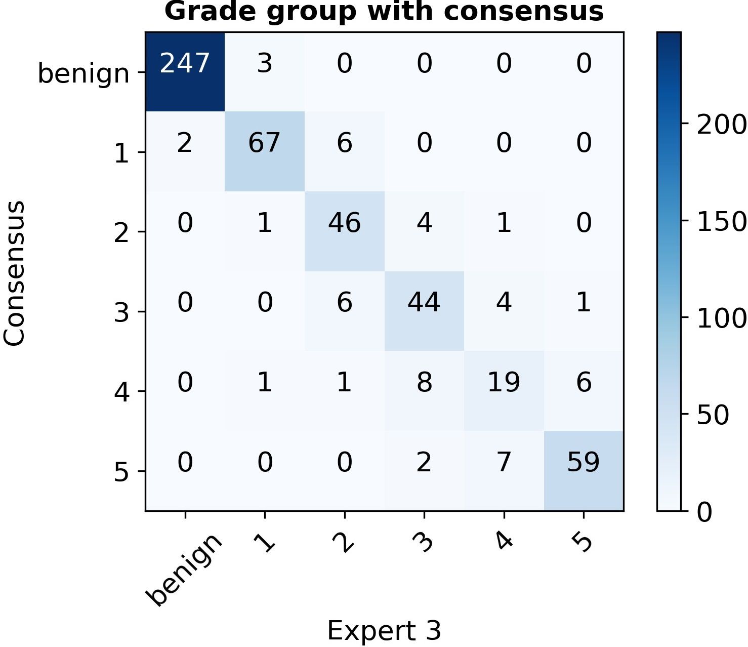
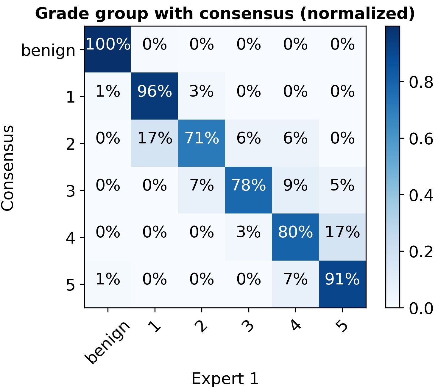
- Confusion matrices experts with consensus on test set
- Supplementary methods
- Tumor detection system
- Epithelium segmentation system
- Overview of deep learning system
- Determining the Gleason grade group for a new specimen
- CycleGAN for style transformation and application to external data
- Determining Gleason score for the external dataset
- Statistical analysis
- References
Abstract
The Gleason score is the strongest correlating predictor of recurrence for prostate cancer, but has substantial inter-observer variability, limiting its usefulness for individual patients. Specialized urological pathologists have greater concordance; however, such expertise is not widely available. Prostate cancer diagnostics could thus benefit from robust, reproducible Gleason grading. We aimed to investigate the potential of deep learning to perform automated Gleason grading of prostate biopsies.
In this retrospective study, we developed a deep-learning system to grade prostate biopsies following the Gleason grading standard. The system was developed using randomly selected biopsies, sampled by the biopsy Gleason score, from patients at the Radboud University Medical Center (pathology report dated between Jan 1, 2012, and Dec 31, 2017). A semi-automatic labeling technique was used to circumvent the need for manual annotations by pathologists, using pathologists’ reports as the reference standard during training. The system was developed to delineate individual glands, assign Gleason growth patterns, and determine the biopsy-level grade. For validation of the method, a consensus reference standard was set by three expert urological pathologists on an independent test set of 550 biopsies. Of these 550, 100 were used in an observer experiment, in which the system, 13 pathologists, and two pathologists in training were compared with respect to the reference standard. The system was also compared to an external test dataset of 886 cores, which contained 245 cores from a different center that were independently graded by two pathologists.
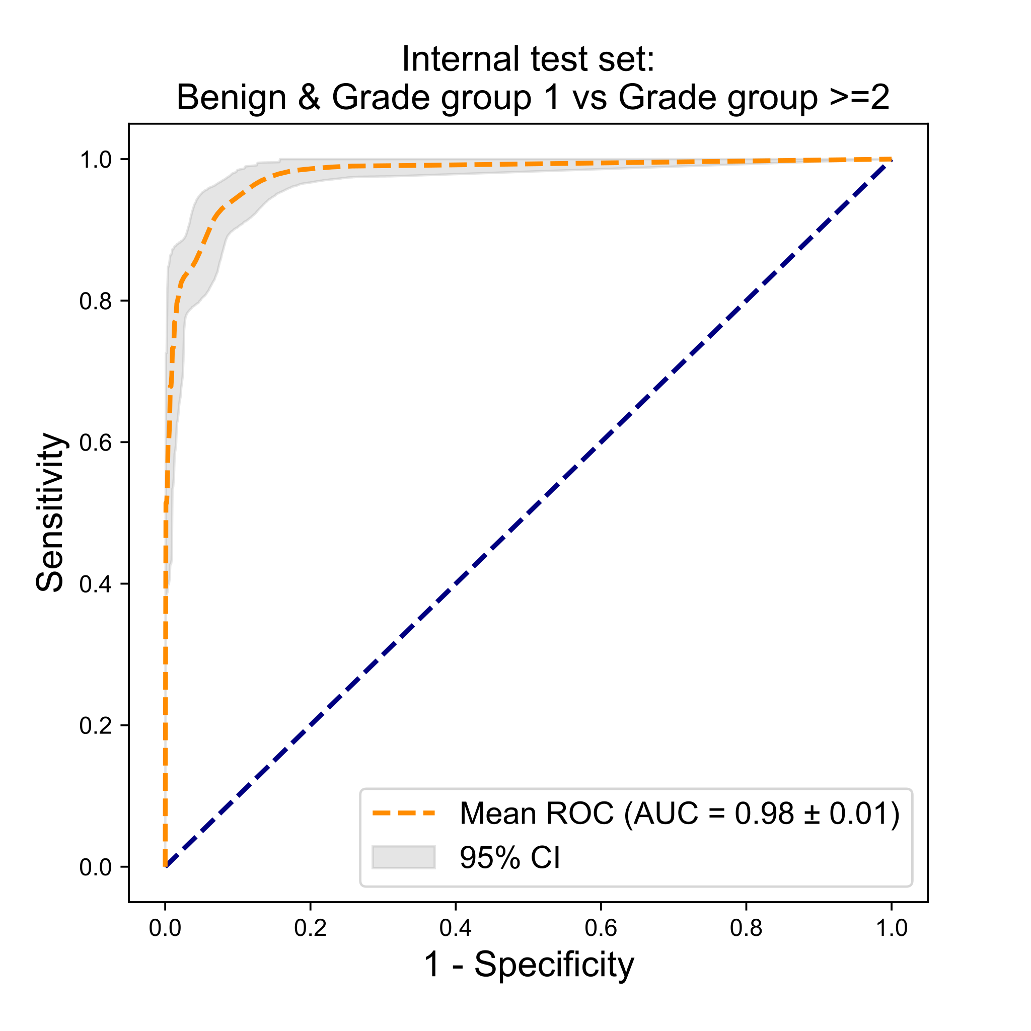
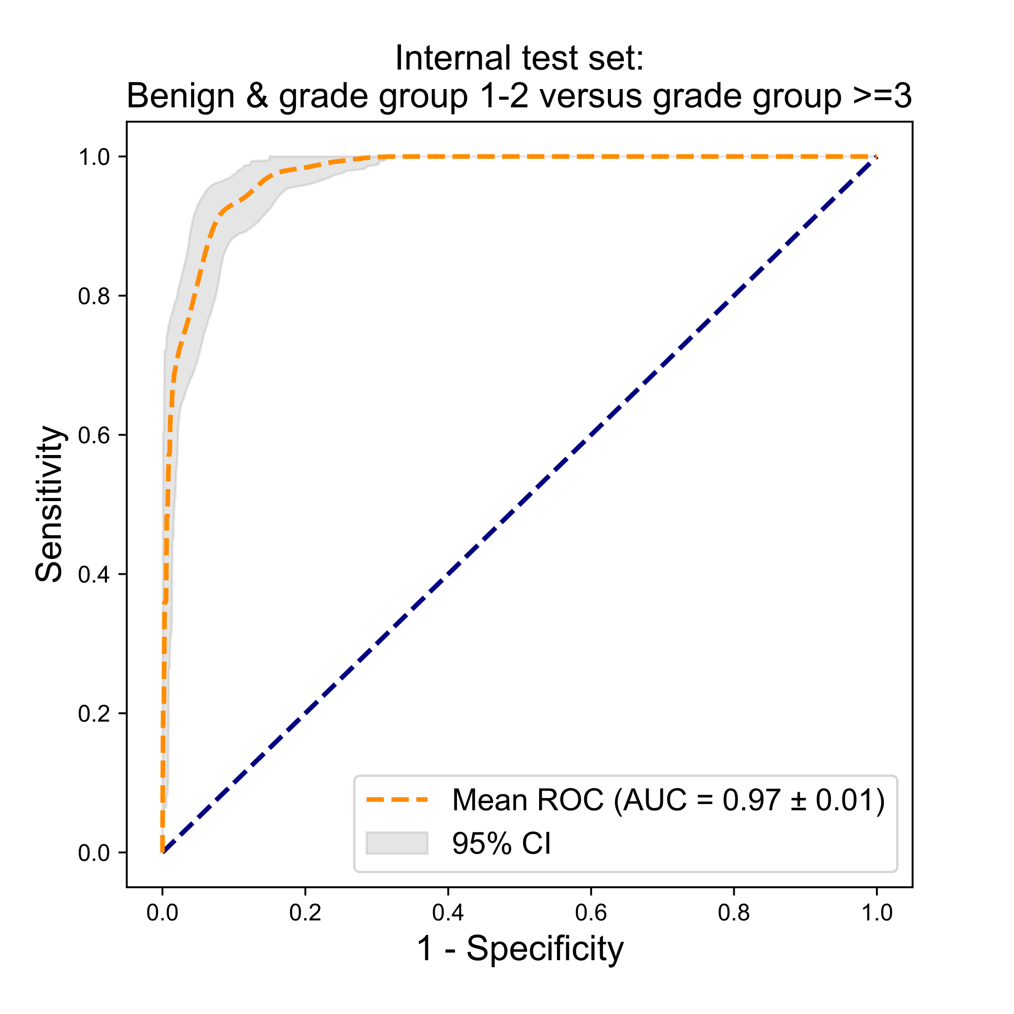
We collected 5759 biopsies from 1243 patients. The developed system achieved a high agreement with the reference standard (quadratic Cohen’s kappa 0·918, 95% CI 0·891–0·941) and scored highly at clinical decision thresholds: benign versus malignant (area under the curve 0·990, 95% CI 0·982–0·996), grade group of 2 or more (0·978, 0·966–0·988), and grade group of 3 or more (0·974, 0·962–0·984). In an observer experiment, the deep-learning system scored higher (kappa 0·854) than the panel (median kappa 0·819), outperforming 10 of 15 pathologist observers. On the external test dataset, the system obtained a high agreement with the reference standard set independently by two pathologists (quadratic Cohen’s kappa 0·723 and 0·707) and within inter-observer variability (kappa 0·71).
Our automated deep-learning system achieved a performance similar to pathologists for Gleason grading and could potentially contribute to prostate cancer diagnosis. The system could potentially assist pathologists by screening biopsies, providing second opinions on grade group, and presenting quantitative measurements of volume percentages.
Introduction
With 1.2 million new prostate cancer cases each year worldwide,1 a high incidence-to-mortality ratio, and risk of overdiagnosis and overtreatment,2 an accurate assessment of patient prognosis is needed. The Gleason score,3 assigned by a pathologist after microscopic examination of cancer morphology, is the most powerful prognostic marker for patients with prostate cancer. However, substantial inter-observer and intra-observer variability in grading45 reduces its usefulness for individual patients. Specialized urological pathologists have greater concordance,6 but such expertise is not widely available. Prostate cancer diagnostics could thus benefit from robust, reproducible Gleason grading.
Treatment planning for prostate cancer is based mainly on the biopsy Gleason score. After the biopsy procedure, tissue specimens are formalin-fixed and paraffin-embedded, cut into thin sections, stained with hematoxylin and eosin, and examined under a microscope by a pathologist. The Gleason system stratifies the architectural patterns of prostate cancer into five types, from 1 (low risk) to 5 (high risk). The Gleason score in biopsies is the sum of the most common pattern and the highest secondary pattern (e.g., 3+5). Growth patterns 1 and 2 are not or rarely reported for biopsies.7
In the latest revision of the Gleason grading system, five prognostically distinct grade groups were introduced;8 assigning scores 3+3 and lower to group 1, 3+4 to group 2, 4+3 to group 3, 3+5, 5+3, and 4+4 to group 4, and higher scores to group 5. Although clinically relevant, initial research shows that this transition has not reduced the observer variability of the grading system.910
Artificial intelligence, particularly deep learning, has the potential to increase the quality of Gleason grading by improving consistency and offering expert-level grading independent of location. Deep learning has already been investigated and shown promising use in diagnostics in several medical fields,11 with examples in radiology,12 ophthalmology,13 dermatology,14 and pathology.15 For prostate cancer, previous studies have applied feature-engineering approaches to address Gleason grading.1618 Eventually, the field transitioned to applications of deep learning for detecting cancer,1920 and later Gleason grading of tissue microarrays,21 prostatectomies,10 and biopsies.22 Studies of biopsies have focused solely on Gleason 3 versus Gleason 4 in small datasets.
We aimed to produce a fully automated cancer detection and Gleason grading system for entire prostate biopsies, trained without the need for manual pixel-level annotations, focusing on the full range of Gleason grades, and evaluated on a large cohort of patients with an expert consensus reference standard, a separate observer study, and an external tissue microarray test dataset.
Methods
Study design and participants
For method development and validation, we retrospectively built several distinct datasets: the internal training, tuning, test, and observer datasets and the external training and test datasets (Figure 3.1).
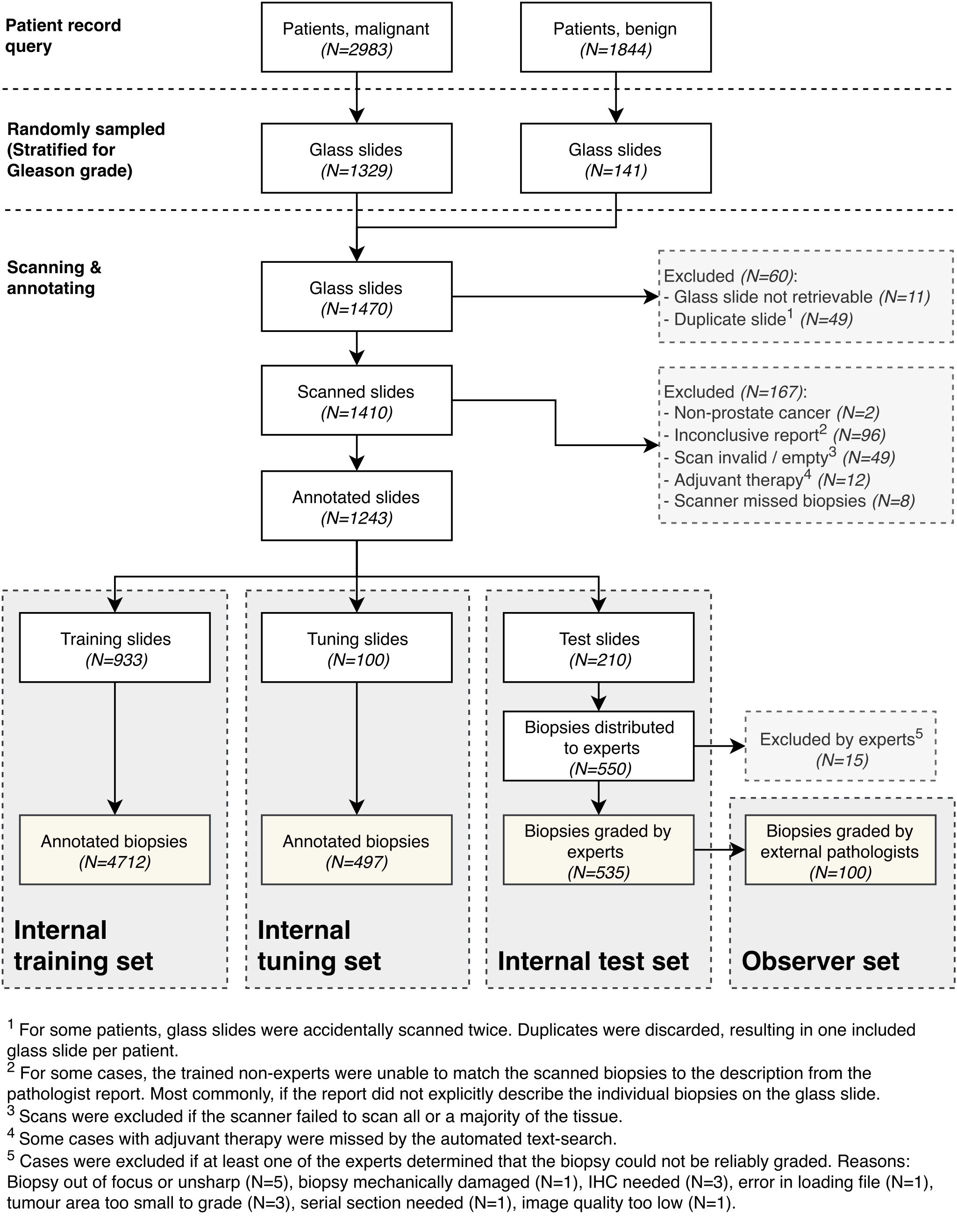
From digital patient records of the Radboud University Medical Center, all pathologist reports dated between Jan 1, 2012, and Dec 31, 2017, for patients who underwent a prostate biopsy owing to a suspicion of prostate cancer were retrieved. The need for informed consent was waived by the local ethics review board (2016–2275). The reports were anonymized, and a text search was used to establish the highest mentioned Gleason score in each report. Patient reports were then randomly sampled using the train_test_split function of the scikit-learn Python package (version 0.20.2), stratifying by the Gleason score, resulting in an equal distribution of Gleason scores. Each pathology report was read, and for each patient, a single hematoxylin and eosin-stained glass slide containing the most aggressive or prevalent part of the tumor was selected for scanning. Additional reports mentioning only benign biopsies were selected. Patients who had neoadjuvant or adjuvant therapy were excluded. The resulting dataset is further referenced to as the internal dataset.
The selected glass slides were scanned using a 3DHistech Pannoramic Flash II 250 (3DHistech, Hungary) scanner at 20× magnification (pixel resolution 0·24 µm). Each scan contained one to six unique biopsies, commonly with two sections per biopsy. After scanning, trained non-experts assessed all slides and coarsely outlined each biopsy, assigning each with a Gleason score or labeling negative on the basis of the pathology report. A fixed number of slides were randomly assigned into datasets for testing or tuning, and the remainder were assigned to the training dataset. Randomization was stratified by patient and highest Gleason grade.
From the internal test dataset, a subset of 100 biopsies was selected to be presented to a group of pathologists in an observer experiment, further referenced to as the observer dataset. The size of the observer dataset was decided in consultation with experts (HvB, RV, and CHvdK). One of the expert pathologists (CHvdK) selected 20 benign cases manually, controlling for a broad range of tissue patterns, including inflammation and (partial) atrophy. The remaining 80 biopsies were randomly selected, stratified for Gleason grade group on the basis of the reported values of the same pathologist.
The 100 biopsies were made available through an online viewer, PMA.view (Pathomation, Berchem, Belgium), and distributed to an external panel. Panel members were invited to participate in this study at the United States and Canadian Academy of Pathology 2019 annual meeting in Washington, DC, USA (March 16–21, 2019). Interested pathologists were asked to report their current affiliation, their experience with Gleason grading, and the number of cases they viewed annually, and were subsequently asked to invite colleagues in their network who had experience in Gleason grading. All pathologists who graded all 100 biopsies were included. All panel members had experience with Gleason grading, but with a varying amount of experience. No time restriction was given, although we asked that they complete the grading within 6 weeks.
We also evaluated the system on an external, independent, public dataset of tissue microarrays21 to assess the robustness of the system to data from a different center (Department of Pathology and Molecular Pathology, University Hospital Zurich, Switzerland).23 One tissue core of a representative tumor area per patient was taken from an online database, and every sample that was assigned to the test dataset of Arvaniti and colleagues21 was used for validation, a total of 245 cores. The complete dataset consisted of 886 tissue cores, each corresponding to a single patient. The cases were prepared and stained in an independent lab and scanned using a different scanner. We had no influence on the composition of and made no changes to the external dataset.
Test methods
The data acquisition of the internal dataset resulted in outlined biopsies with a single label per biopsy. More detailed annotations were required to train the deep-learning system to segment individual glands. We preprocessed the biopsies of the training and tuning set in four steps (Figure 3.2). First, tissue was automatically distinguished from background using a tissue segmentation network.24 Second, within tissue areas, a trained tumor detection system19 was applied to define a rough outline of the tumor. The outlined tumor regions still contained large areas of stroma, inflammation, or other non-epithelial tissue. Third, to refine the tumor masks, each biopsy was processed by an epithelial tissue detection system,25 after which tissue that was detected as non-epithelial tissue was removed from the tumor mask. Finally, detected tumor tissue was assigned a label on the basis of the Gleason score retrieved from the pathology report. A description of the individual systems is provided in the supplementary methods.
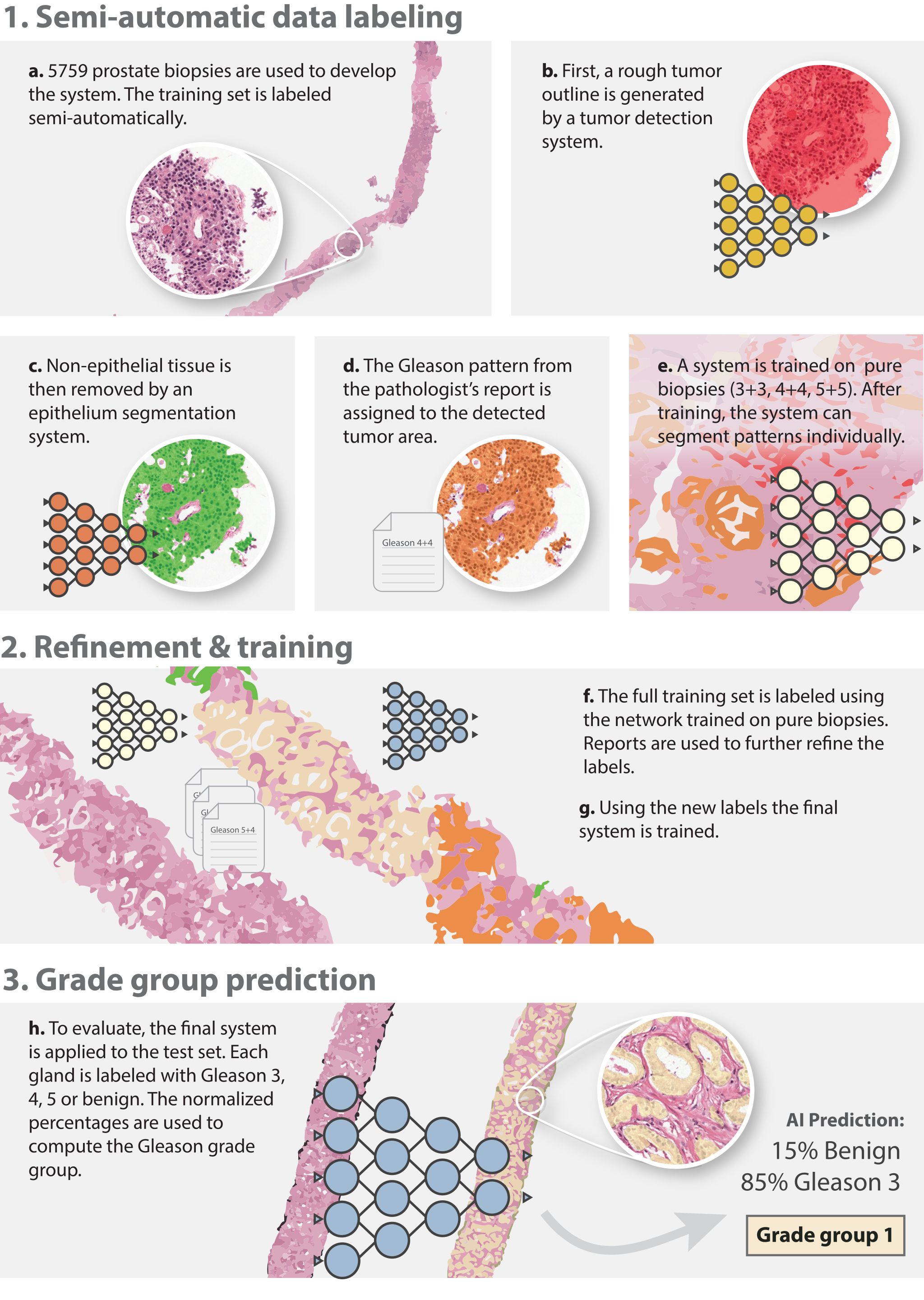
We first trained a deep-learning system only on biopsies with a pure Gleason score (3+3, 4+4, or 5+5).26 After training, this initial system was applied to the internal training dataset to set the reference standard. By use of the pathologist reports, the output was automatically refined by removing clearly incorrect label assignments, such as cancerous glands in benign biopsies. Any tissue originating from benign biopsies detected as malignant was relabelled as hard negative (i.e., a sample of benign tissue that was difficult for the system to correctly classify) to be oversampled during training. A connected components algorithm, based on the ndimage.label function from the Python SciPy package (version 1.2.1), was applied to ensure that each gland was assigned to a single class.
The patients included in the internal test dataset were independent of the patients in the internal training and tuning datasets. To create a strong reference standard, we asked three pathologists with a subspecialty in urological pathology (CHvdK, HvB, and RV) to grade the biopsies individually through the online viewer, PMA.view, following the International Society of Urological Pathology 2014 guidelines.27 Clinical information of the patients was not available for the experts.
The reference standard for the internal test dataset was determined in three rounds. In the first round, each pathologist reviewed the biopsies individually. For positive biopsies, each pathologist was asked to report: primary, secondary, and tertiary Gleason grade (if present), total tumor volume, tumor volumes for the growth patterns, and the Gleason grade group. In the second round, each biopsy without consensus was regraded by the pathologist whose score differed from the other two. Additional to the pathologist’s initial examination, the Gleason scores of the other pathologists were appended anonymously. Biopsies without consensus after round two were discussed in a consensus meeting.
Our deep-learning system consisted of an extended U-Net28 that was trained on patches extracted from the internal training dataset. After the aforementioned semi-automatic labeling process, the system was trained on the complete training dataset, including biopsies with mixed Gleason growth patterns. The tuning dataset was used to monitor performance during training and to prevent overfitting. Training of the system was halted if no performance increase was measured on the tuning dataset.
The label quality of the internal training dataset was determined by labeling the test cases using the same automated method. We compared the retrieved Gleason scores of the test dataset with the final consensus score of the experts. The kappa values of this comparison acted as a measure of label quality.
After training, the deep-learning system was applied to all biopsies from the test dataset and compared with the reference standard. Test positivity cutoffs were determined before the analysis of the test dataset using the tuning dataset. The system determined the grade group of a biopsy in two steps. In the first step, the whole biopsy was segmented by assigning Gleason growth patterns to tumorous glands, and benign glands are classified as benign. From this segmentation, a normalized ratio of epithelial tissue could be calculated as percentages of benign, grade 3, grade 4, or grade 5. Based on the tuning dataset, we classified a biopsy as malignant if at least 10% of the epithelial tissue was predicted as cancer by the system. In the second step, the grade group was determined on the basis of the normalized volume percentages of each growth pattern.
To apply the system to the external dataset and to account for stain and scanner variations, we applied an unsupervised normalisation algorithm based on CycleGANs.29 After normalization of the external test images, our deep-learning system, without any modification, was applied to the normalized test images. The reference standard for the external test dataset was based on the Gleason score. To account for this difference in test metrics, we determined test positive cutoffs on the external training data. For the external test dataset, no consensus score was available for the two pathologists who graded all cases; instead, we evaluated our method using both pathologists in turn as the reference standard.
Statistical analysis
After consultation with experts (HvB, RV, and CHvdK), 550 cases for the test dataset was established as a good balance between time investment and case diversity.
We defined the main metric as the agreement with the consensus reference standard, measured using quadratic Cohen’s kappa. To compare the performance of the system with the external panel of pathologists, we did multiple permutation tests. The test statistic was defined as the difference between the kappa of the deep-learning system and the median kappa of the pathologists. The analysis of the receiver operating characteristic curves was done using the difference in F1 score as test metric. Statistical analysis was done using Python 3.6 with the NumPy (1.16.3), pandas (0.25.1), scipy (1.2.1), scikit-learn (0.20.2) and matplotlib (2.2.4) packages. Further details are provided in the supplementary methods.
Role of the funding source
The funder of the study had no role in study design, data collection, data analysis, data interpretation, or writing of the report. The corresponding author had full access to all the data in the study and had final responsibility for the decision to submit for publication.
Results
Dataset & reference standard
After screening of 1329 slides from patients with malignant disease and 141 slides from patients with benign disease, 1410 slides were scanned. After exclusion of 167 slides, the internal dataset consisted of 1243 patients and 5759 biopsies. The training dataset consisted of 933 (75%) of 1243 slides (4712 biopsies), the tuning dataset of 100 (8%) of 1243 slides (497 biopsies), and the test dataset of 210 (17%) of 1243 slides (550 biopsies; Figure 3.1). The observer dataset was sampled from the test dataset and consisted of 100 biopsies from 78 patients.
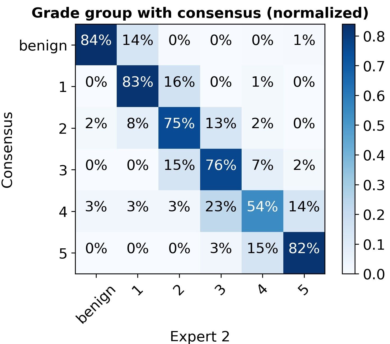
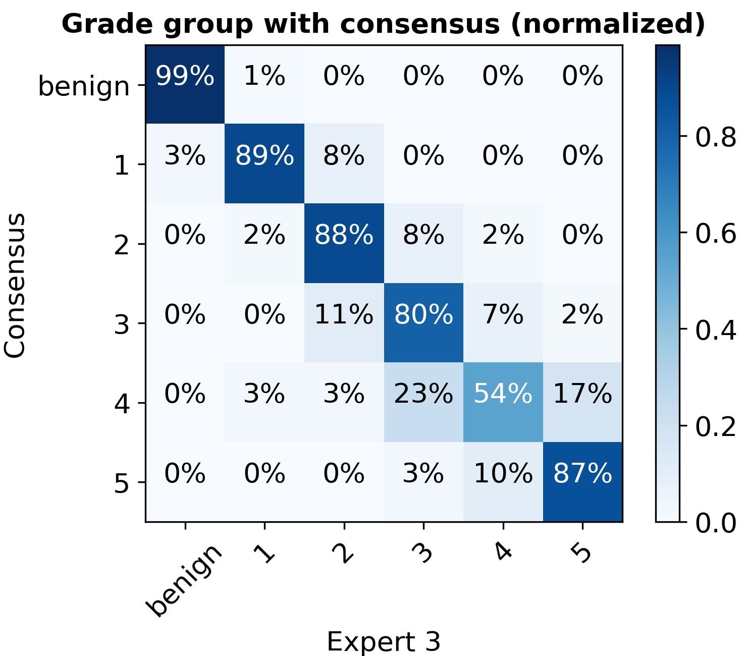
After the first round of grading of biopsies in the internal test dataset, 333 (61%) of 550 cases had complete consensus. The three experts’ inter-rater agreement was high (quadratic Cohen’s kappa of 0·925). The majority vote was taken for some slides: 11 (2%) of 550 cases with an agreement on grade group, but a difference in Gleason pattern order (eg, 5+4 versus 4+5); 11 (2%) cases with an equal grade group, but a disagreement on Gleason score; and 110 (21%) cases for which two pathologists agreed and the third had a maximum deviation of one grade group. Cases with a disagreement on malignancy were always flagged for a second read. Immunohistochemistry was used in seven (1%) of 550 cases to determine the benign or malignant label as it was present in the original report. 15 (3%) of the 550 cases were excluded by the experts because they could not be reliably graded. In the second round, 63 (11%) of 550 cases were regraded. 27 (5%) of 550 cases of biopsies without consensus after round two were discussed in a consensus meeting. Grade group distribution and confusion matrices are presented in Supplementary Figure 3.
To get an estimate of label noise, the reference standard was compared with labels generated by the semi-automatic method; the accuracy of the retrieved labels versus the reference was 0·675 (kappa 0·819) for Gleason score and 0·720 (kappa 0·853) for grade group.
Performance on the internal test set
On the 535 biopsies of the internal test dataset, our deep-learning system achieved an agreement of 0·918 (quadratic Cohen’s kappa, 95% CI 0·891–0·941) with the consensus grade group. Most errors by the deep-learning system are made in distinguishing between grade group 2 and 3, and grade group 4 and 5 (Figure 3.3).
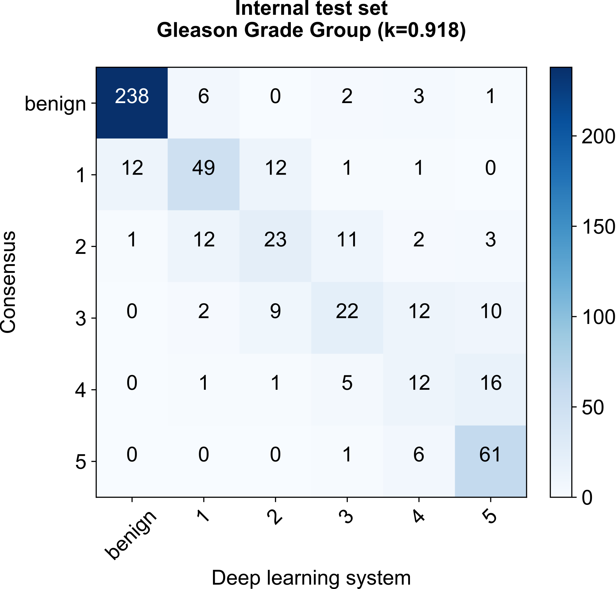
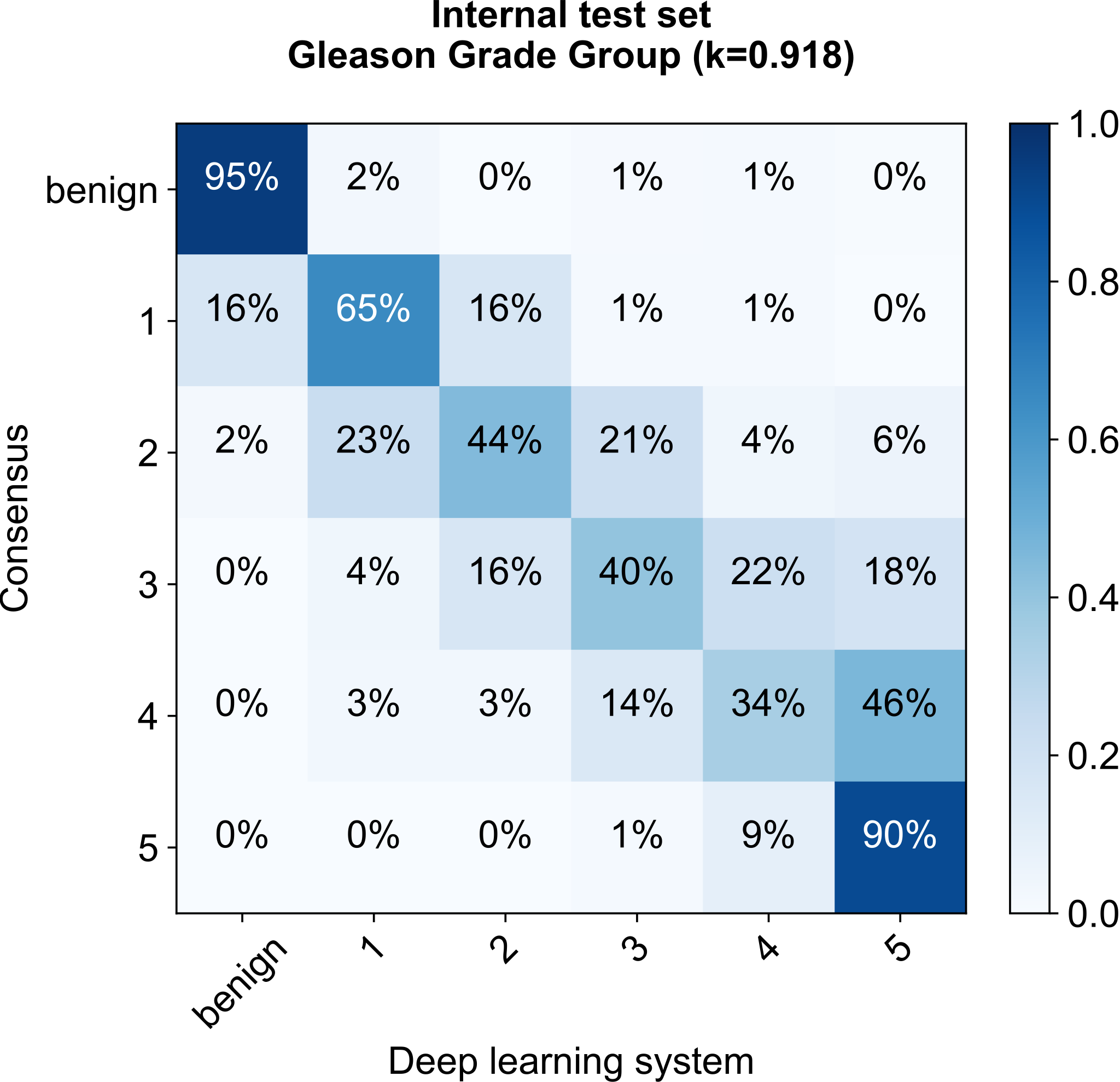
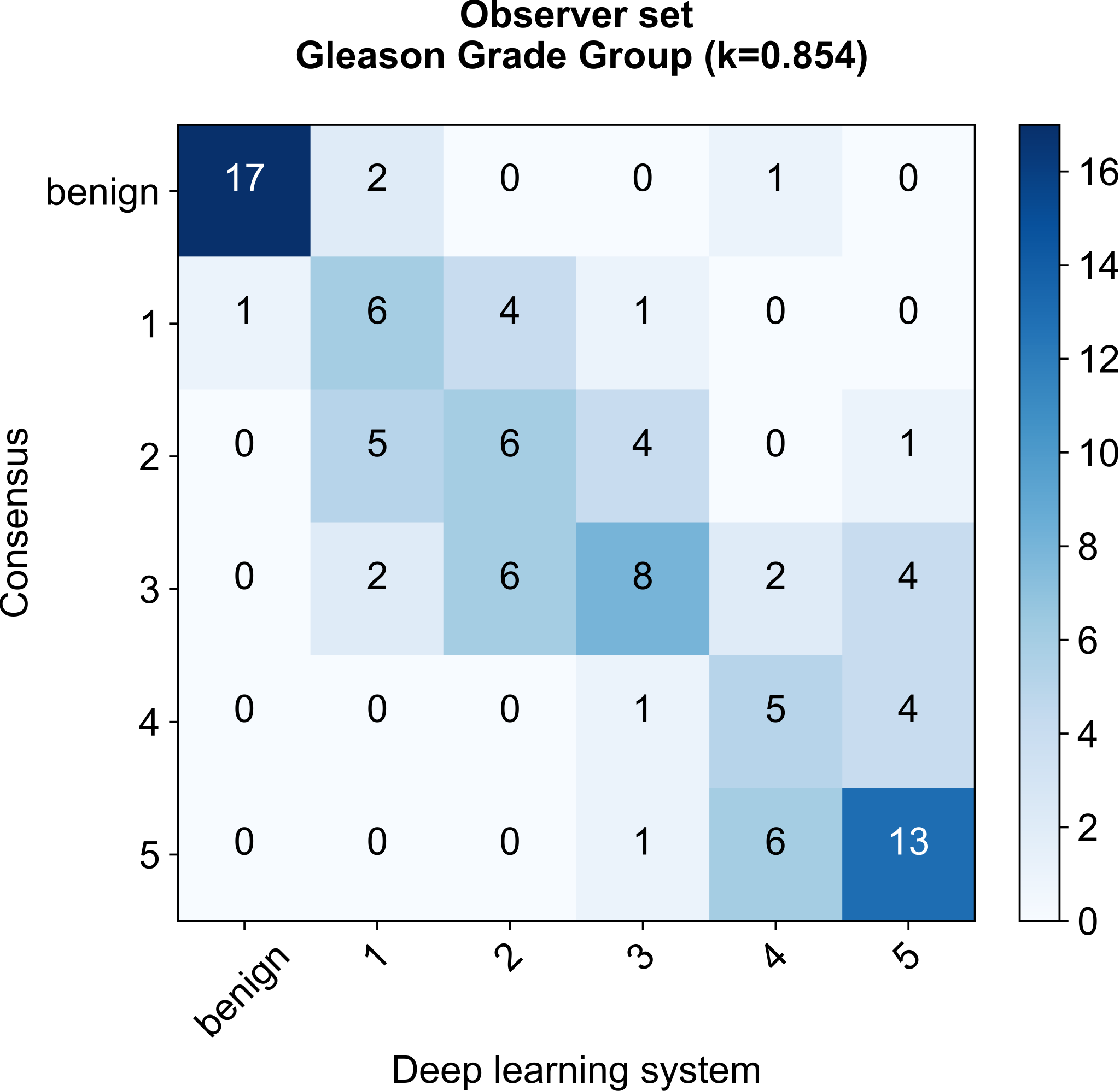
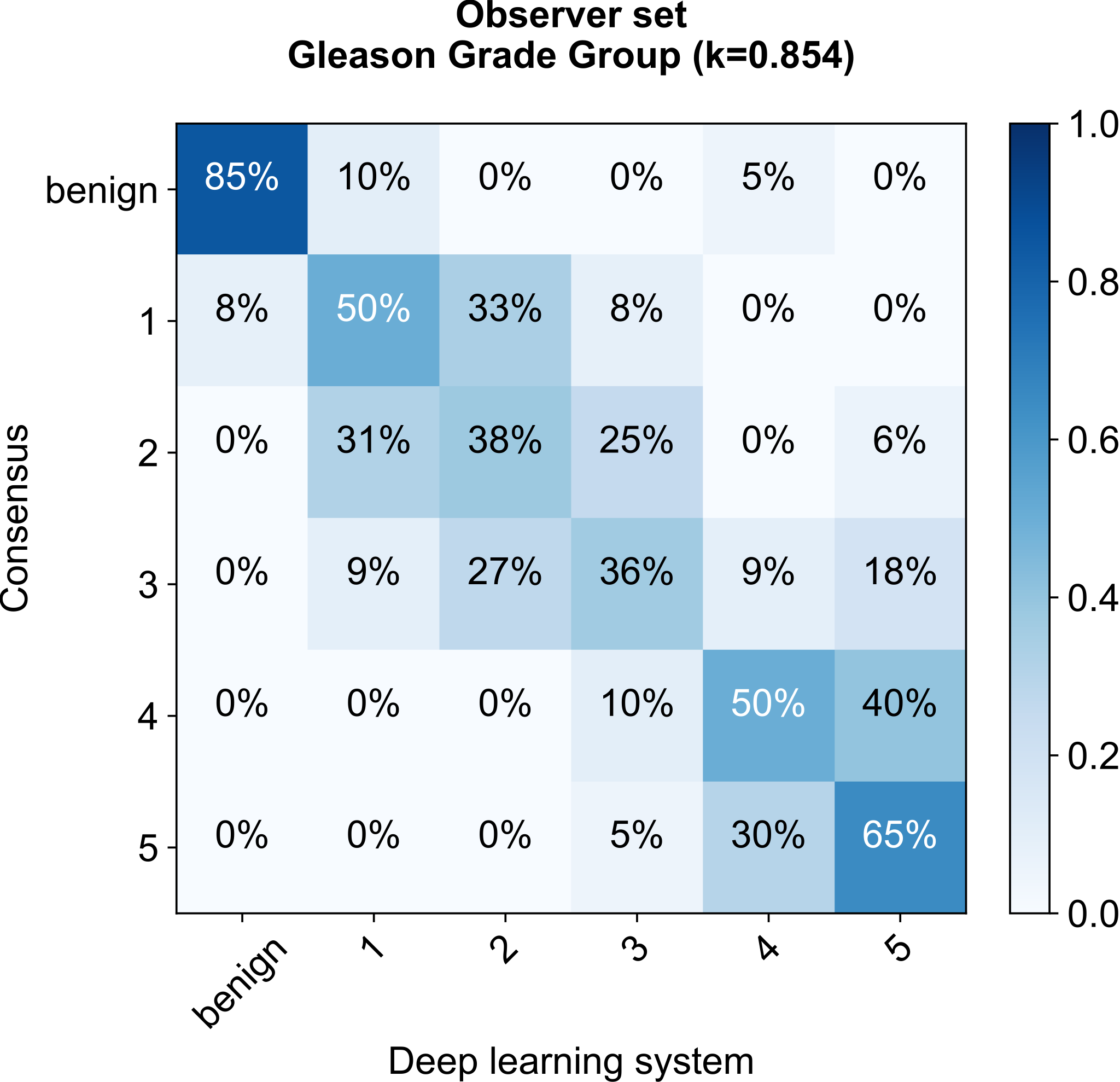
In the internal test dataset, the deep-learning system missed 13 malignant cases, of which all but one were determined as grade group 1 by the experts (Figure 3.3a). In 12 of these cases, the system detected a tumor, but the predicted volume was below our threshold for malignancy.
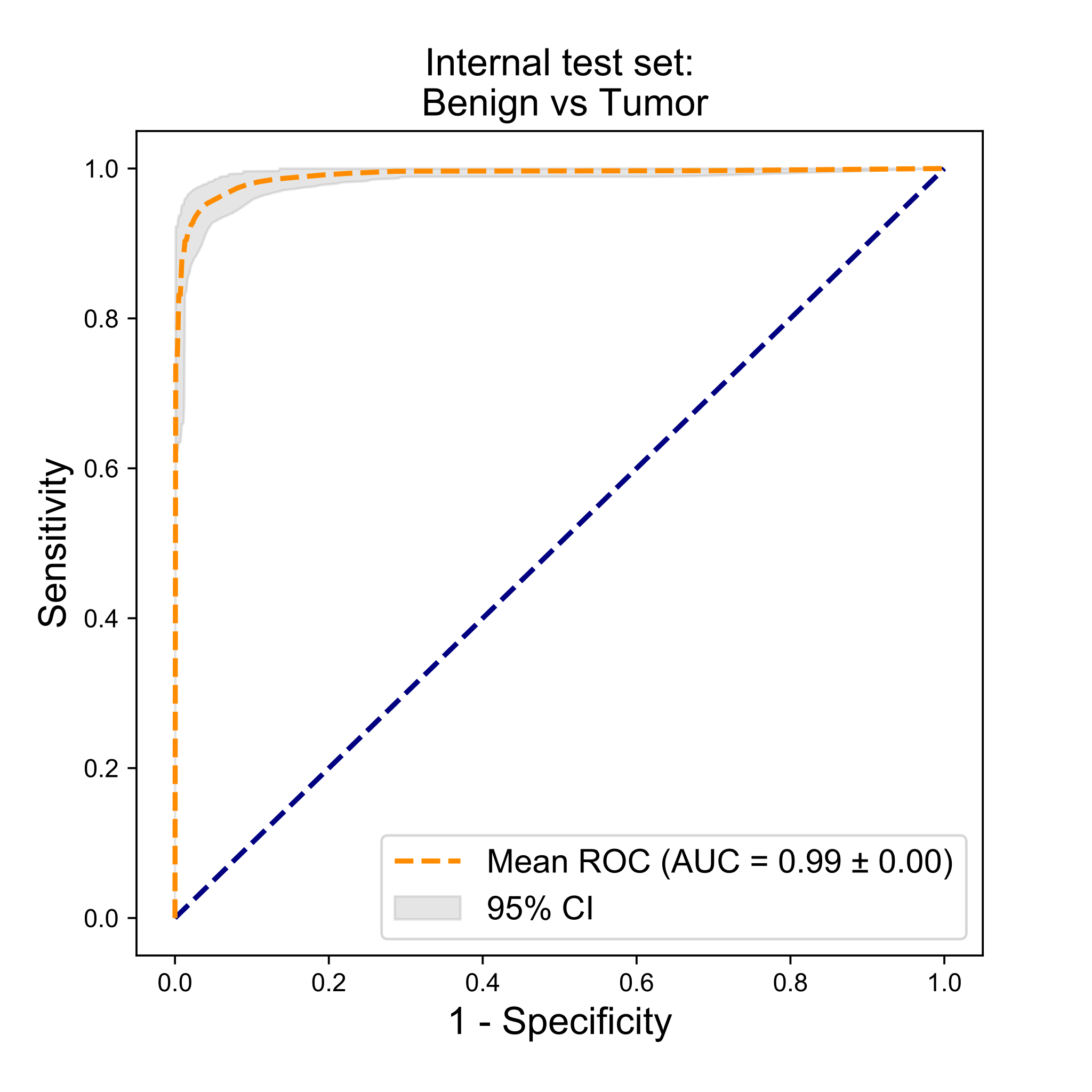
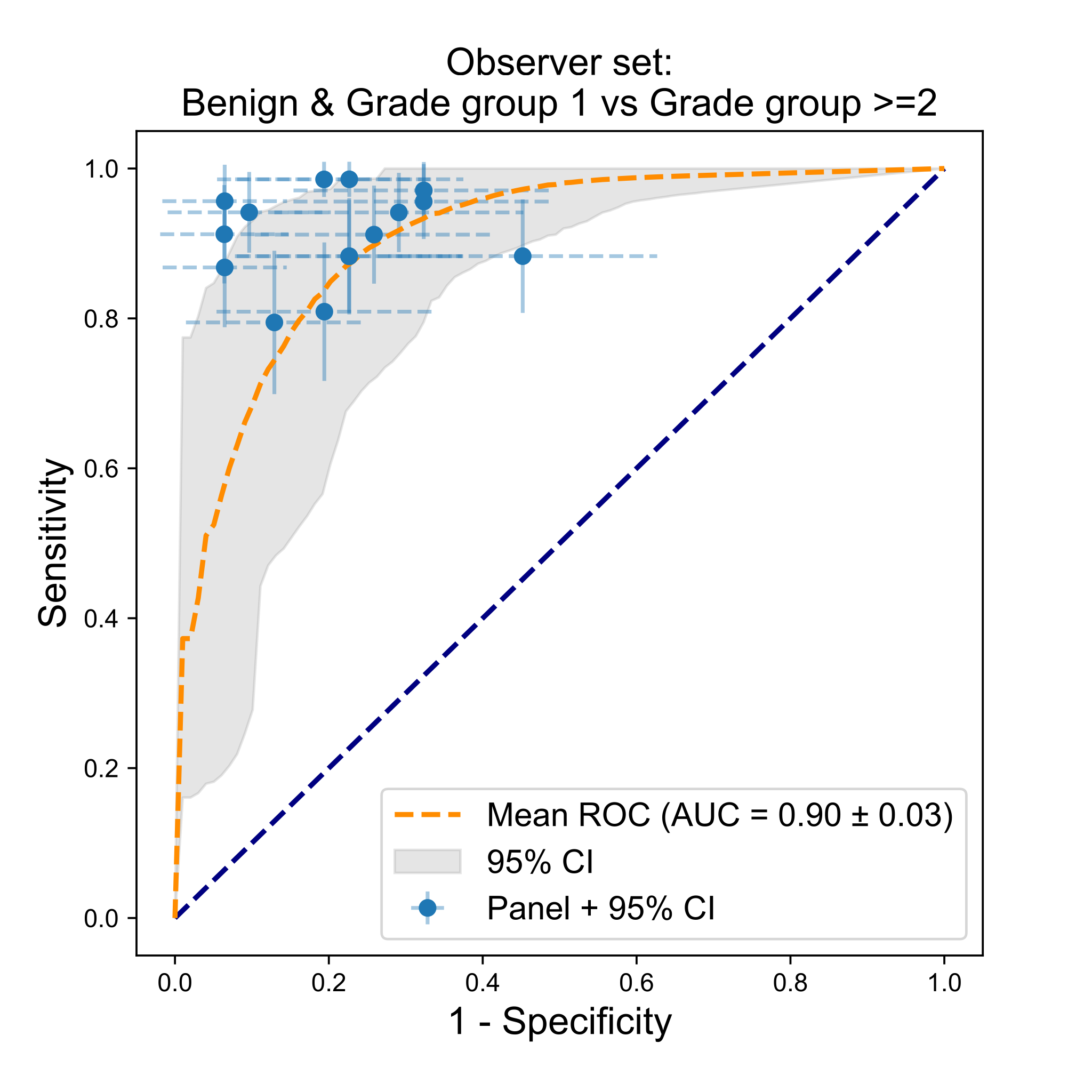
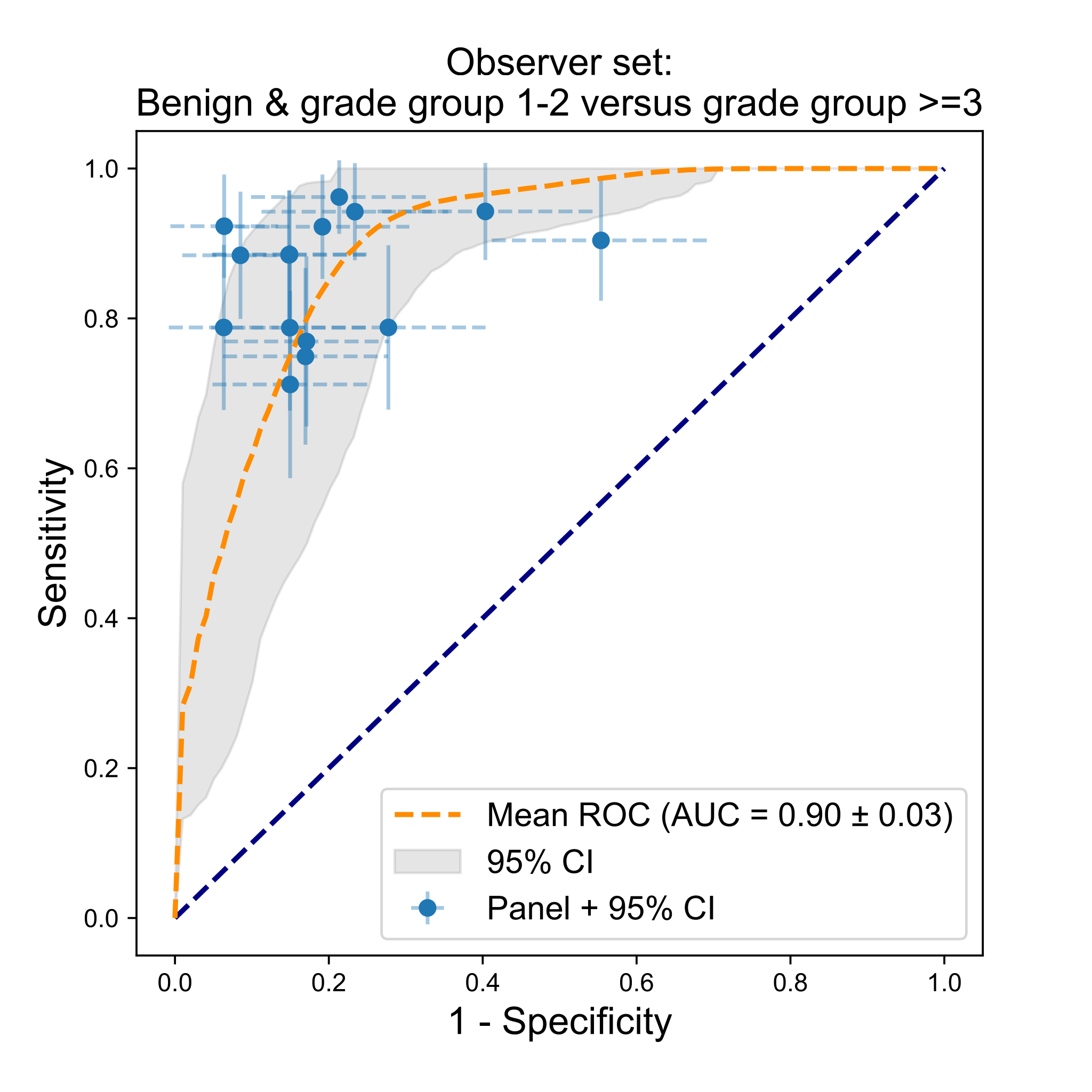
Receiver operating characteristic curve analysis on three clinically relevant cutoffs showed the ability of the system to group cases in risk categories with high accuracy (Figure 3.4a, 3.5a and 3.6a). The decision threshold of the system can be tuned to correctly predict 99% of biopsies containing tumor with a specificity of 82%.
Comparison to a panel of pathologists
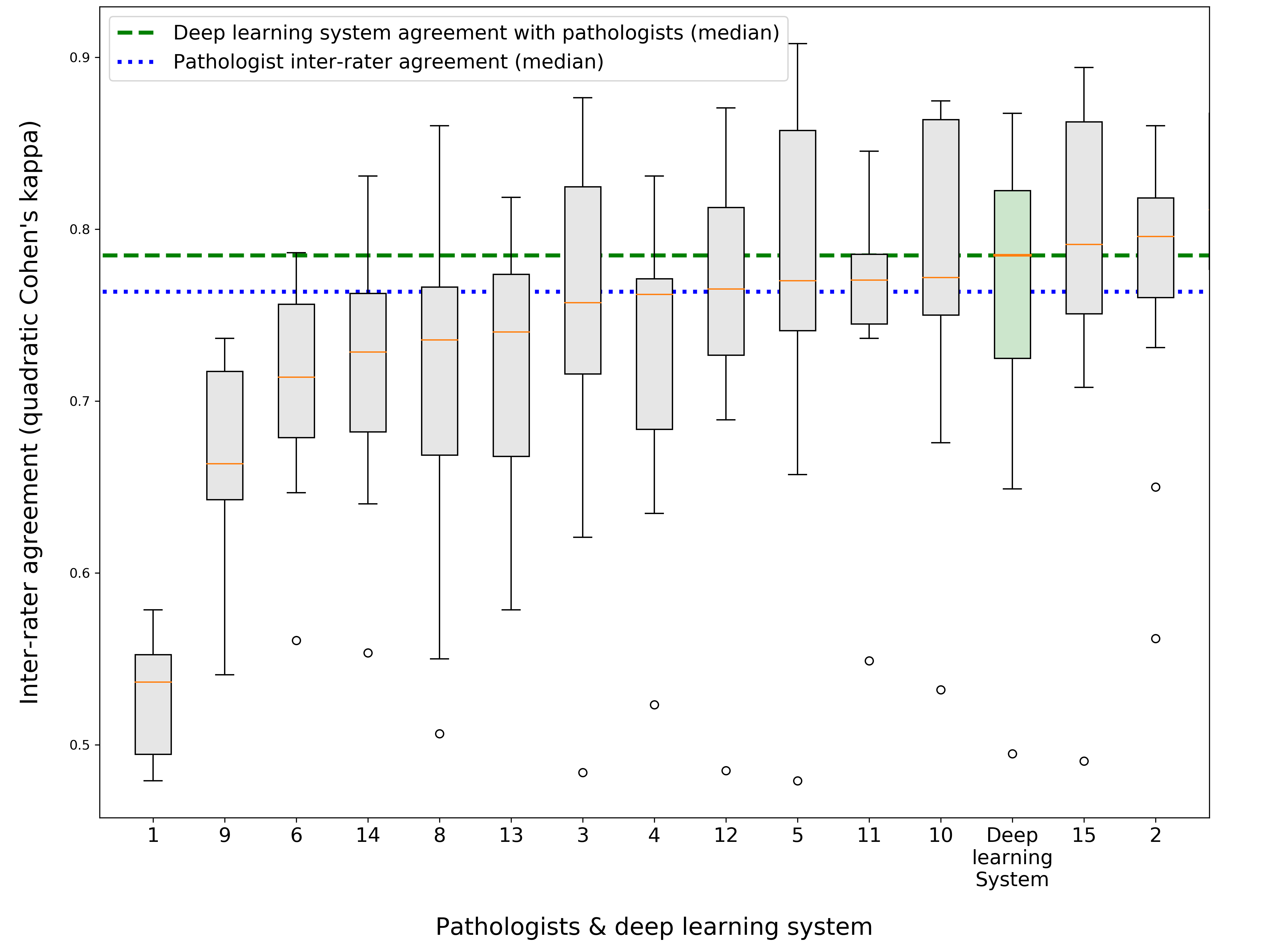
For the observer study, 13 pathologists and two pathologists in training from 14 independent labs and ten countries individually graded all 100 biopsies following the International Society of Urological Pathology 2014 guidelines. This external panel showed a median inter-rater agreement of 0·819 (quadratic kappa, 95% CI 0·726–0·869) on Gleason grade group with the consensus (Figure 3.7). The system achieved a kappa value of 0·854 (quadratic kappa, 0·777–0·914) on the cases of the observer dataset, scoring higher than the median value of the panel and outperforming 10 of the 15 panel members (Figure 3.7). The performance of the deep-learning system was better than that of pathologists with less than 15 years of experience (two-sided permutation test, p=0·036) and scores not significantly different than pathologists with more than 15 years of experience (two-sided permutation test, p=0·96). To exclude bias towards the experts in our results, we computed the inter-rater agreement between all panel members independently of the reference standard. We then computed the agreement of the system with all members of the panel (Supplementary Figure 1). Sorted by the median kappa value, the deep-learning system had the third-highest inter-rater agreement score.
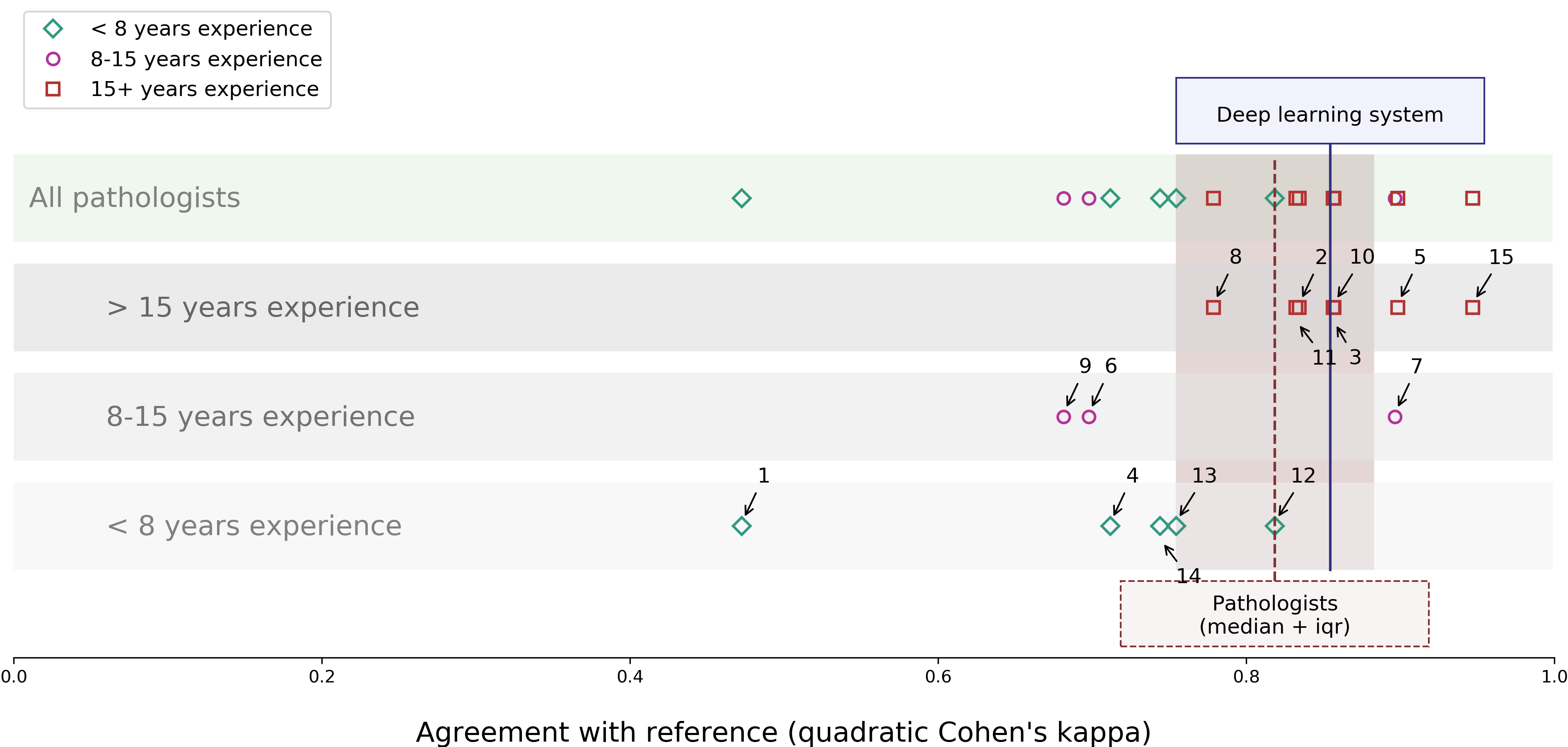
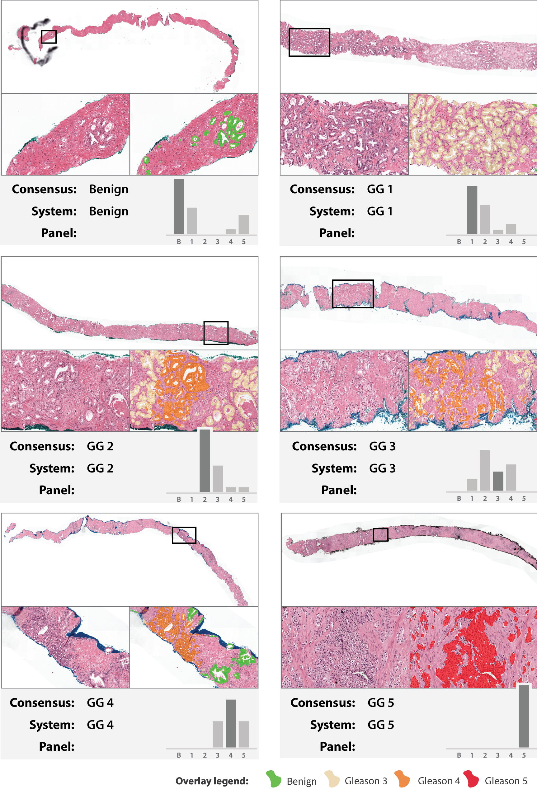
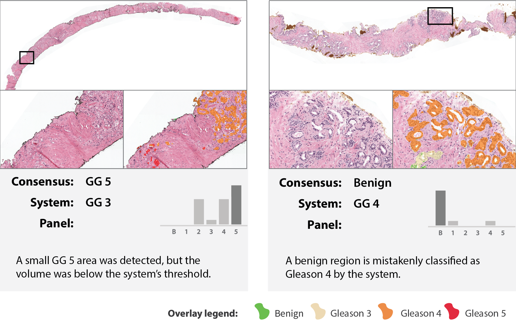
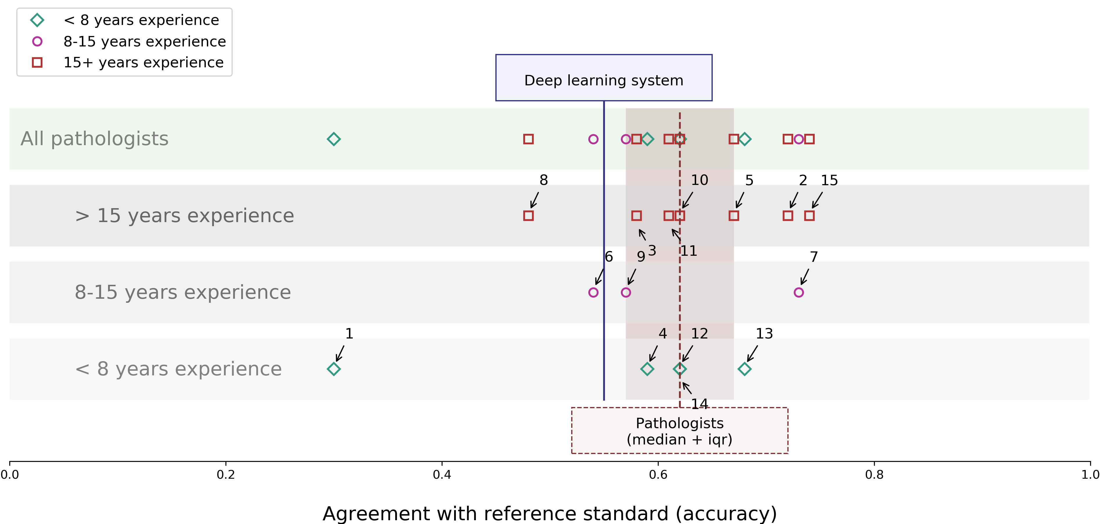
The deep-learning system scores better than three pathologists of the panel but lower than most on accuracy (Supplementary Figure 2). The lower accuracy is mostly caused by one-off errors between grade groups 2 versus 3 and 4 versus 5 (Figure 3.3). A two-sided permutation test on the difference between system accuracy and the median of the panel showed no significant difference (p=0·15). See Figure 3.8 for example cases.
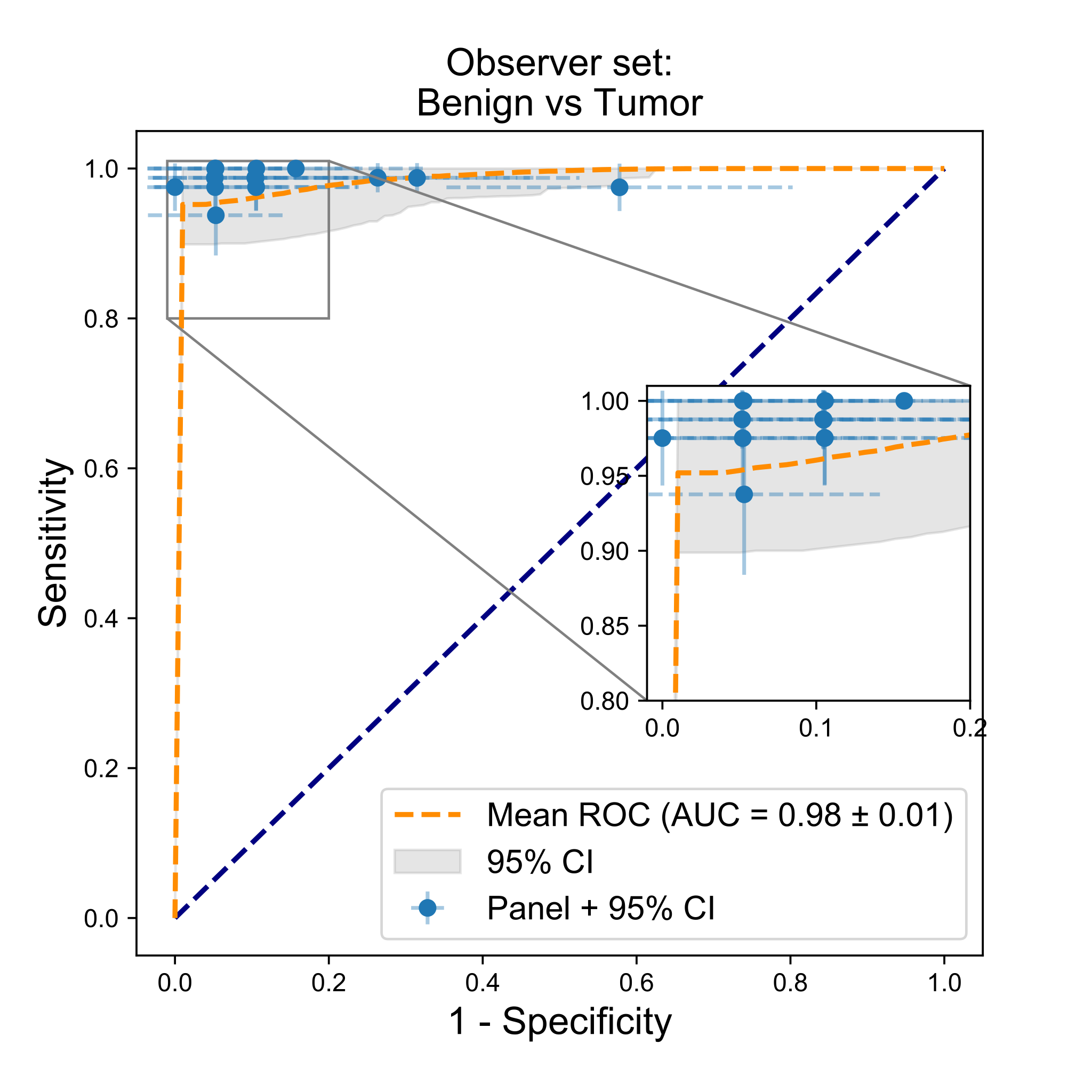
After receiver operating characteristic analysis of the observer dataset, a two-sided permutation test on the median F1 score showed no difference between the deep-learning system and the panel for both malignant versus benign (p=0·70), grade group 2 as a cutoff (p=0·84), and grade group 3 as a cutoff (p=0·65; Figure 3.4b, 3.5b and 3.6b).
Performance on the external test set
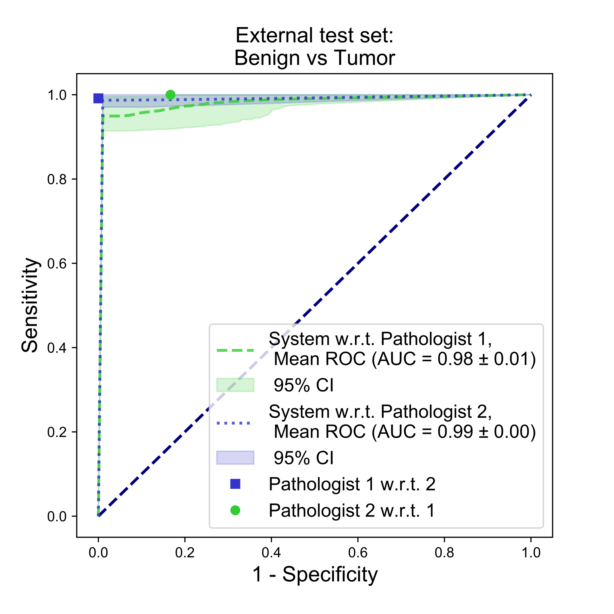
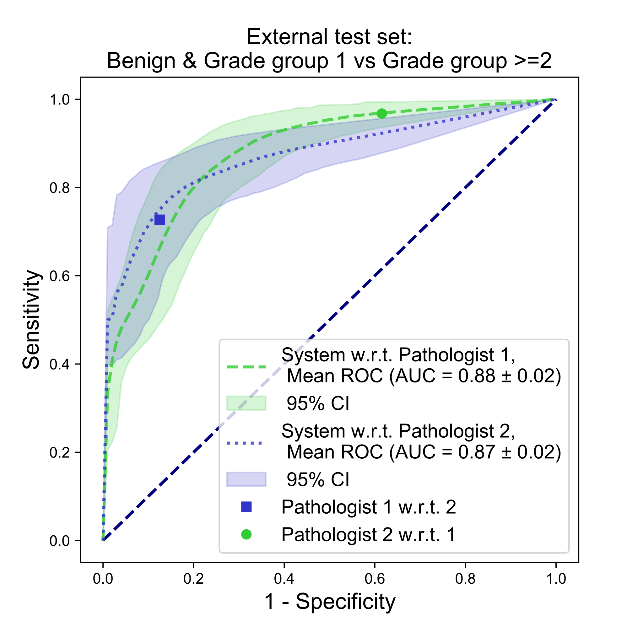
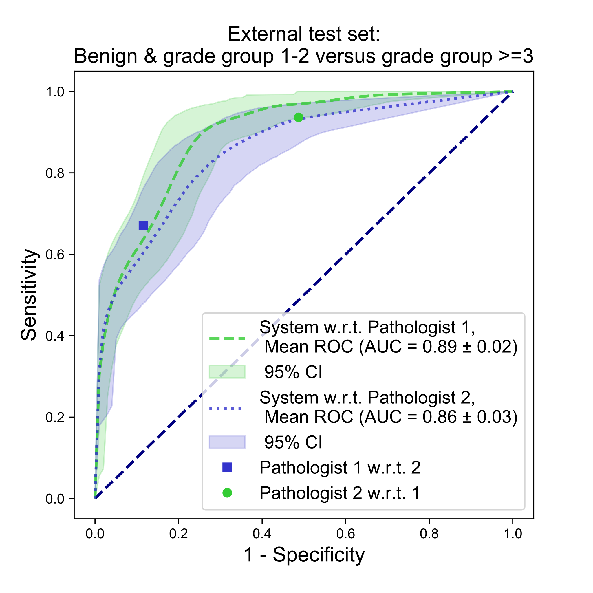
The external test dataset contained 245 cores that were independently graded by two pathologists (inter-rater agreement quadratic Cohen’s kappa 0·71). Concerning the two pathologists, the system obtained a 0·723 and 0·707 quadratic kappa on Gleason score. A receiver operating characteristic analysis for relevant decision thresholds was also done for the external test set (Figure 3.9). Overall, the deep learning system performed comparably to the two pathologists who set the reference standard.
Discussion
We have developed a fully automated method to grade prostate biopsies and have shown that this method can achieve a performance similar to pathologists on both the internal and external test datasets. The performance of the deep-learning system could only reliably be assessed by use of an expert reference standard. We asked three expert urological pathologists to grade the complete test dataset, which resulted in a minimum of three independent reads for every case. The deep-learning system achieved a high agreement (quadratic kappa of 0·918) with the reference standard. We also compared the system with a panel of independent pathologists and pathologists in training. In this observer dataset, the deep-learning system outperformed ten of 15 panel members. On the external test dataset, the system showed it could generalize to external and unseen data. The system scored comparably to the results attained by Arvaniti and colleagues21 (quadratic kappa, 0·723 and 0·707 vs 0·71 and 0·75) and within inter-observer variability of the pathologists who set the reference standard (kappa 0·71), although our system was not trained on data from that set.
The training data was labelled in a semi-supervised way, saving resources that would otherwise have been spent in manually labeling slides. Moreover, it is often practically unfeasible to precisely annotate the vast amounts of data required for deep learning, even though unannotated or sparsely annotated data is often readily available in pathology archives. One limitation of this method is that it can introduce label noise in the training dataset. However, the ability of deep-learning systems to handle substantial amounts of label noise is well known.30
The black-box characteristic of deep learning is often mentioned as a drawback of such systems, especially for medical decision making. We addressed this drawback by having our system show predictions at multiple abstraction levels, instead of using an additional learned model on top of the deep-learning system. The precise gland-level segmentations of the developed system made it possible to use a simple ruleset on grade volume percentages to obtain the biopsy-level grade, similar to the one described in the Gleason grading system. This approach allows pathologists to assess whether the epithelium was correctly classified, whether the system missed certain glands, and the grades assigned to individual or groups of glands. As such, our system provides a higher level of interpretability compared with competing approaches.10
Given the high prevalence of prostate cancer, reducing workload for pathologists is of clinical value. In the test dataset, our deep-learning system achieved an AUC of 0·990 on determining the malignancy of a biopsy, on the observer set an AUC of 0·984. Furthermore, the system can be tuned to achieve a sensitivity of 99%. As such, our system could be implemented as a prescreening triage tool within pathology labs, giving priority to high-grade biopsies and filtering out low-risk benign biopsies.
More work is needed to increase the discrimination power of the system between Gleason grade groups 2 and 3 and groups 4 and 5. The boundaries between group 2 and 3 are defined by the relative volume percentages of the Gleason growth patterns, which makes an accurate estimate of those volumes essential for correct classification. Group 4 versus 5 is complicated by a wide range of Gleason scores that fall under these two groups (3+5, 5+3, 4+4, 4+5, 5+4, and 5+5). Discrepancies can also be related to the way the system and pathologists differ in estimating the relative volume of growth patterns. The system counts the exact area of the individual glands, whereas a pathologist assesses the volume more qualitatively. Some failure cases of the system are shown in Figure 3.10.
Our results extend previous work on prostate cancer detection1920 and automated Gleason grading.102122 We extend on these works by focusing on automated Gleason grading for prostate biopsies, the strongest histological correlating predictor of recurrence for patients with prostate cancer, of which the grading system differs from prostatectomies. Furthermore, by including both benign biopsies and biopsies from the full spectrum of Gleason grades, we created a system that is usable as a prescreening tool and as a second reader.
Grading of the biopsies, both by the experts and the external panel, was done through digital viewing of the slides. For the external panel, not all members had previous experience with digital viewing or with the digital viewer used in this study. Owing to this inexperience, we cannot know whether it affected their grading. Nonetheless, research has shown that digital viewing is non-inferior to microscopy.31
Before our system can be used in clinical practice, some limitations must be addressed. First, the data that were used to develop the deep-learning system originated from a single center. Although the performance on the external test dataset is within the range of inter-observer variability, including data from multiple centers, with different staining protocols and whole slide scanners, could further increase the robustness of the system. Second, we focused on the grading of acinar adenocarcinoma in prostate biopsies, although other tumor types and foreign tissue can be present in prostate biopsies (eg, colon glands, which should be identified and excluded for grading). Additionally, other prognostic information could be present in the biopsies that we did not extract (eg, the detection of intraductal carcinoma).32 Finally, in this study, each biopsy is treated independently, both by the pathologists and by the deep-learning system. In clinical practice, multiple biopsies are sampled from different regions of the prostate. An update to the deep-learning system could take multiple biopsies into account and give a grade group prediction at the patient level.
The developed system will be made available for scientific and non-commercial use, through the Radboudumc Computational Pathology Group website. Furthermore, through a grand challenge on Gleason grading, we will publish a part of our data for others to use in developing new methods for automated Gleason grading.
Our automated deep-learning system achieved a performance similar to pathologists in terms of Gleason grading. With further evaluation, the system could assist pathologists by screening biopsies, providing second opinions on grade group, and presenting quantitative measurements of volume percentages.
Acknowledgements
This study was funded by a grant from the Dutch Cancer Society (KWF), grant number KUN 2015-7970.
We would like to thank the following pathologists and pathologists in training for participating in our study as part of the panel:
- Paulo G. O. Salles, M.D. Ph.D. MBA, Instituto Mário Penna, Belo Horizonte, Brazil;
- Vincent Molinié, M.D., Ph.D., CHU de Martinique, Université des Antilles, Fort de France, Martinique;
- Jorge Billoch-Lima, M.D. FCAP, HRP Labs, San Juan, Puerto Rico;
- Ewout Schaafsma, M.D., Ph.D., Radboud University Medical Center, Nijmegen, The Netherlands;
- Anne-Marie Vos, M.D., Radboud University Medical Center, Nijmegen, The Netherlands;
- Xavier Farré, M.D., Ph.D., Department of Health, Public Health Agency of Catalonia. Lleida, Catalonia, Spain.
- Awoumou Belinga Jean-Joël, M.D., Ph.D. Candidate, Department of Morphological Sciences and Anatomic Pathology, Faculty of Medicine and Biomedical Sciences, University of Yaounde 1, Cameroon;
- Joëlle Tschui, M.D., Medics Pathologie, Bern, Switzerland;
- Paromita Roy, M.D., Tata Medical Center, Kolkata, India;
- Emílio Marcelo Pereira, M.D., Oncoclínicas group, Brazil;
- Asli Cakir, M.D., Pathologist, Istanbul Medipol University School of Medicine, Pathology Department, Istanbul, Turkey;
- Katerina Geronatsiou, M.D., center de Pathologie, Hopital Diaconat Mulhouse, France;
- Günter Saile, M.D., Histo- and Cytopathology, labor team w ag, Goldach SG, Switzerland;
- Américo Brilhante, M.D., SalomãoZoppi Diagnostics, São Paulo, Brazil;
- Guilherme Costa Guedes Pereira, M.D., Laboratory Histo Patologia Cirúrgica e Citologia, João Pessoa-PB, Brazil.
We also thank Jeffrey Hoven for assisting with the data collection and scanning, and Milly van de Warenburg, Nikki Wissink, and Frederike Haverkamp for their help making the manual annotations.
Supplementary figures
Grade group agreement (quadratic kappa) between panel and deep learning system
Accuracy deep learning system accuracy versus panel
Confusion matrices experts with consensus on test set
Supplementary methods
Tumor detection system
A previously developed tumor detection system was applied19 to outline tumor areas in our training set. To train this tumor detection system, a pathologist in training, supervised by an experienced uropathologist, outlined tumor regions in 100 prostate biopsies. Most of these biopsies were low grade: 52 benign, 11 grade group 1, 23 grade group 2, seven grade group 3, five grade group 4, and two biopsies grade group 5. The biopsies used for the development of the tumor detection system were independent of the biopsies used in the current study.
Patches were extracted from the 100 biopsies and used to train the system (pixel resolution of 1.92µm). The tumor detection system achieved an AUC of 0.99 in discriminating benign from malignant biopsies on a separate test set of 75 biopsies.
After training, the system was applied as a fully convolutional network to all biopsies of the current study. This procedure resulted in a rough outline of tumor regions.
Epithelium segmentation system
A previously developed epithelium segmentation system25 was used to refine the tumor outlines generated by the tumor detection system. The epithelium segmentation system was developed using 102 prostatectomy tissue sections. The tissue sections were stained with H&E and subsequently restained with P63 and CK8/18 immunohistochemistry (IHC) markers to highlight epithelial structures. Each H&E and IHC pair were subsequently co-registered.
An initial deep learning system was trained on a subset of the IHC slides that were preprocessed with color deconvolution. This trained system was then applied to all IHC slides in the training set, forming a reference standard for the final system. This automated labeling method made sure that even poorly differentiated Gleason 5 areas were precisely annotated.
The final epithelium segmentation system was trained on the H&E slides using the automatically generated reference standard. A five-level-deep U-Net28 was used as the network architecture with patches extracted at a pixel resolution of 0.98µm. The system achieved a high segmentation performance (F1 score of 0.893) and was able to segment both intact glands and individual malignant epithelial cells.
Overview of deep learning system
Our deep learning system consisted of a U-Net28 that was trained on randomly sampled patches extracted from the training set. After the automatic labeling process, the system could be trained on all biopsies, including those with mixed Gleason growth patterns. Additional patches were sampled from the hard-negative areas to improve the system’s ability to distinguish tumor from benign tissue.
We followed the original U-Net architecture but experimented with different configurations. Given the importance of morphological features in Gleason grading, we focused on multiple depths of the U-Net, combined with different pixel spacings for the training data. Experimentation showed the best performance on the tuning set using a depth of six levels, sampled patches with a size of 1024×1024, and a pixel resolution of 0.96 µm. We added additional skip connections within each layer block and used up-sampling operations in the expansion path. Adam optimization was used with β₁ and β₂ set to 0.99, a learning rate of 0.0005 and a batch size of 8. The learning rate was halved after every 25 consecutive epochs without improvement on the tuning set. We stopped training after 75 epochs without improvement on the tuning set. Adding additional training examples from hard negative areas increased the performance of the network, especially in distinguishing between benign, inflammatory, and tumorous tissue.
The network was developed using Keras33 and TensorFlow.34 Data augmentation was used to increase the robustness of the network. The following augmentation procedures were used: flipping, rotating, scaling, color alterations (hue, saturation, brightness, and contrast), alterations in the H&E color space, additive noise, and Gaussian blurring.
Determining the Gleason grade group for a new specimen
Our deep learning system determines the Gleason grade group for a biopsy in two steps. First, our trained U-Net is applied to the scanned tissue of the biopsy. This procedure results in a label for each pixel of the image: background, stroma, benign epithelium, Gleason 3, Gleason 4, or Gleason 5. The frequency of each label can then be counted. Biopsies can differ vastly in size and in the amount of epithelial tissue that is present. To account for this difference, the values for the three Gleason growth patterns are normalized based on the sum of benign and malignant epithelial tissue. By normalizing, we obtain a volume estimate of the tumor that is independent of the size of the biopsy.
The volume percentages were used to assign a Gleason score and Gleason Grade group based on the guidelines for biopsies in clinical practice.27 First, we determine whether a biopsy is malignant or benign. Based on the tuning set, we classify a biopsy as malignant if at least 10% of the epithelial tissue is predicted as cancer by the system. For malignant biopsies, we then determine the Gleason score. The growth pattern that has the largest volume is taken as the primary component. If there are other growth patterns present, with a volume of at least 7%, the most aggressive component is used as the secondary pattern. The 7 and 10% cut-offs were determined automatically based on the tuning set. Note that this procedure differs between prostatectomies and biopsies. For prostatectomies, the secondary pattern is always the second-largest growth pattern, regardless of aggressiveness.
The predicted Gleason score is used to determine the grade group. A Gleason score 3+3 is mapped to group 1; Gleason score 3+4 is mapped to group 2; Gleason score 4+3 is mapped to group 3; Gleason scores 3+5, 4+4 and 5+3 are mapped to group 4; and higher scores are mapped to Gleason 5.
CycleGAN for style transformation and application to external data
We used a cycle-consistent generative adversarial network (CycleGAN)35 system to facilitate stain transformation on the external dataset of tissue microarrays. In a CycleGAN setup, two separate networks are trained to perform a transformation from one stain to the other, while retaining the structural information of the tissue. We used a previously developed CycleGAN setup that was developed for the transformation of histopathological tissue.29 The CycleGAN was adapted to learn the residual change instead of reconstructing the full image.
To train the CycleGAN system, we sampled patches from the internal training set and used the full external dataset. Before inference with the Gleason deep learning system, we applied the CycleGAN network on the whole external dataset. The CycleGAN network was implemented in TensorFlow.34
Determining Gleason score for the external dataset
The original paper of the external dataset21 reports the quadratic kappa on Gleason score as the primary metric. The Gleason scores were determined using the standard for grading prostatectomies: the sum of the most and second most common growth patterns. We applied our algorithm to the test set of this paper and computed the quadratic kappa on Gleason score to allow a one-to-one comparison of our algorithm to the algorithm developed by Arvaniti et al. To account for the difference in the grading systems between prostatectomies and biopsies, we adjusted the decision thresholds of the deep learning system using the training data set of 641 cores, resulting in a tumor threshold of 3% and a secondary pattern threshold of 1.5%.
Statistical analysis
To compare the performance of the deep with the external panel of pathologists, we performed multiple permutation tests. The permutation test was implemented as follows: For each case in the observer set, we obtained a list of predictions, one by the deep learning system and the remainder by the pathologists. In each iteration of the permutation test, for each case, we swapped the grade group prediction of the system with a random prediction from the list of predictions. After swapping the predictions, the test statistic was computed. Repeating this procedure 10.000 times resulted in a null distribution of the test statistic. The original test statistic was then compared to the null distribution, resulting in a two-tailed p-value.
We defined the main metric as the agreement with the consensus reference standard, measured using quadratic Cohen’s kappa. For the analysis on agreement with the reference, we defined the test statistic as the difference between the kappa of the deep learning system and the medium kappa of the pathologists. The panel of pathologists was split into two groups, those with less than 15 years experience and those with more, and a permutation test was performed for both groups. The analysis of the ROC curves was done using the difference in F1-score as the metric. The decision threshold for the system was based on the point that maximized the AUC. The comparison of grade group accuracy was made using the difference in the accuracy of the system and the median accuracy of the pathologists with respect to the reference standard.
References
- Bray F, Ferlay J, Soerjomataram I, Siegel RL, Torre LA, Jemal A. Global cancer statistics 2018: GLOBOCAN estimates of incidence and mortality worldwide for 36 cancers in 185 countries. CA: A Cancer Journal for Clinicians. 2018;68(6):394–424. doi:10.3322/caac.21492
- Schröder FH, Hugosson J, Roobol MJ, Tammela TLJ, Ciatto S, Nelen V, et al. Prostate-cancer mortality at 11 years of follow-up. New England Journal of Medicine. 2012;366:981–990. doi:10.1056/NEJMoa1113135
- Epstein JI. An update of the Gleason grading system. Journal of Urology. 2010;183:433–440. doi:10.1016/j.juro.2009.10.046
- Allsbrook WC, Mangold KA, Johnson MH, Lane RB, Lane CG, Epstein JI. Interobserver reproducibility of Gleason grading of prostatic carcinoma: General pathologists. Human Pathology. 2001;32(1):81–88. doi:10.1053/hupa.2001.21135
- Egevad L, Ahmad AS, Algaba F, Berney DM, Boccon-Gibod L, Compérat E, et al. Standardization of Gleason grading among 337 European pathologists. Histopathology. 2013;62(2):247–256. doi:10.1111/his.12008
- Allsbrook WC, Mangold KA, Johnson MH, Lane RB, Lane CG, Amin MB, et al. Interobserver reproducibility of Gleason grading of prostatic carcinoma: Urologic pathologists. Human Pathology. 2001;32(1):74–80. doi:10.1053/hupa.2001.21134
- Epstein JI, Allsbrook WC, Amin MB, Egevad LL, Bastacky S, López Beltrán A, et al. The 2005 International Society of Urological Pathology (ISUP) consensus conference on Gleason grading of prostatic carcinoma. American Journal of Surgical Pathology. 2005;29(9):1228–1242. doi:10.1097/01.pas.0000173646.99337.b1
- Epstein JI, Zelefsky MJ, Sjoberg DD, Nelson JB, Egevad L, Magi-Galluzzi C, et al. A Contemporary Prostate Cancer Grading System: A Validated Alternative to the Gleason Score. European urology. 2016;69(3):428–435. doi:10.1016/j.eururo.2015.06.046
- Ozkan TA, Eruyar AT, Cebeci OO, Memik O, Ozcan L, Kuskonmaz I. Interobserver variability in Gleason histological grading of prostate cancer. Scandinavian Journal of Urology. 2016;50(6):420–424. doi:10.1080/21681805.2016.1206619
- Nagpal K, Foote D, Liu Y, Chen PHC, Wulczyn E, Tan F, et al. Development and validation of a deep learning algorithm for improving Gleason scoring of prostate cancer. npj Digital Medicine. 2019;2(1):48. doi:10.1038/s41746-019-0112-2
- Litjens G, Kooi T, Ehteshami Bejnordi B, Setio AAA, Ciompi F, Ghafoorian M, et al. A Survey on Deep Learning in Medical Image Analysis. Medical image analysis. 2017;42:60–88. doi:10.1016/j.media.2017.07.005
- Ardila D, Kiraly AP, Bharadwaj S, Choi B, Reicher JJ, Peng L, et al. End-to-end lung cancer screening with three-dimensional deep learning on low-dose chest computed tomography. Nature Medicine. 2019;25(June). doi:10.1038/s41591-019-0447-x
- De Fauw J, Ledsam JR, Romera-Paredes B, Nikolov S, Tomasev N, Blackwell S, et al. Clinically applicable deep learning for diagnosis and referral in retinal disease. Nature medicine. 2018;24(9):1342–1350. doi:10.1038/s41591-018-0107-6
- Esteva A, Kuprel B, Novoa RA, Ko J, Swetter SM, Blau HM, et al. Dermatologist-level classification of skin cancer with deep neural networks. Nature. 2017;542(7639):115–118. doi:10.1038/nature21056
- Ehteshami Bejnordi B, Veta M, van Diest PJ, van Ginneken B, Karssemeijer N, Litjens G, et al. Diagnostic Assessment of Deep Learning Algorithms for Detection of Lymph Node Metastases in Women With Breast Cancer. Journal of the American Medical Association. 2017;318(22):2199–2210. doi:10.1001/jama.2017.14585
- Naik S, Doyle S, Feldman M, Tomaszewski J, Madabhushi A. Gland Segmentation and Computerized Gleason Grading of Prostate Histology by Integrating Low- , High-level and Domain Specific Information. In: Proceedings of 2nd Workshop on Microsopic Image Analysis with Applications in Biology. 2007:1–8.
- Gertych A, Ing N, Ma Z, Fuchs TJ, Salman S, Mohanty S, et al. Machine learning approaches to analyze histological images of tissues from radical prostatectomies. Computerized Medical Imaging and Graphics. 2015;46 Pt 2:197–208. doi:10.1016/j.compmedimag.2015.08.002
- Nguyen TH, Sridharan S, Macias V, Kajdacsy-Balla A, Melamed J, Do MN, et al. Automatic Gleason grading of prostate cancer using quantitative phase imaging and machine learning. Journal of Biomedical Optics. 2017;22(3):036015. doi:10.1117/1.jbo.22.3.036015
- Litjens G, Sánchez CI, Timofeeva N, Hermsen M, Nagtegaal I, Kovacs I, et al. Deep learning as a tool for increased accuracy and efficiency of histopathological diagnosis. Nature Scientific Reports. 2016;6:26286. doi:10.1038/srep26286
- Campanella G, Hanna MG, Geneslaw L, Miraflor A, Werneck Krauss Silva V, Busam KJ, et al. Clinical-grade computational pathology using weakly supervised deep learning on whole slide images. Nature Medicine. 2019. doi:10.1038/s41591-019-0508-1
- Arvaniti E, Fricker KS, Moret M, Rupp N, Hermanns T, Fankhauser C, et al. Automated Gleason grading of prostate cancer tissue microarrays via deep learning. Scientific Reports. 2018;8(1):1–11. doi:10.1038/s41598-018-30535-1
- Lucas M, Jansen I, Savci-Heijink CD, Meijer SL, de Boer OJ, van Leeuwen TG, et al. Deep learning for automatic Gleason pattern classification for grade group determination of prostate biopsies. Virchows Archiv. 2019. doi:10.1007/s00428-019-02577-x
- Zhong Q, Guo T, Rechsteiner M, Rüschoff JH, Rupp N, Fankhauser C, et al. A curated collection of tissue microarray images and clinical outcome data of prostate cancer patients. Scientific data. 2017;4(1):1–9.
- Bandi P, van de Loo R, Intezar M, Geijs D, Ciompi F, van Ginneken B, et al. Comparison of Different Methods for Tissue Segmentation In Histopathological Whole-Slide Images. In: IEEE International Symposium on Biomedical Imaging. 2017:591–595. doi:10.1109/ISBI.2017.7950590
- Bulten W, Bándi P, Hoven J, van de Loo R, Lotz J, Weiss N, et al. Epithelium segmentation using deep learning in H&E-stained prostate specimens with immunohistochemistry as reference standard. Nature Scientific Reports. 2019;9(864). doi:10.1038/s41598-018-37257-4
- Bulten W, Pinckaers H, Hulsbergen-van de Kaa C, Litjens G. Automated Gleason Grading of Prostate Biopsies Using Deep Learning. In: United States and Canadian Academy of Pathology (USCAP) 108th Annual Meeting. 2019.
- Epstein JI, Egevad L, Amin MB, Delahunt B, Srigley JR, Humphrey PA. The 2014 International Society of Urological Pathology (ISUP) Consensus Conference on Gleason Grading of Prostatic Carcinoma. The American Journal of Surgical Pathology. 2016;40(2):1. doi:10.1097/pas.0000000000000530
- Ronneberger O, Fischer P, Brox T. U-Net: Convolutional Networks for Biomedical Image Segmentation. In: Medical Image Computing and Computer-Assisted Intervention. Lecture Notes in Computer Science. Vol 9351. 2015:234–241.
- de Bel T, Hermsen M, Kers J, van der Laak J, Litjens G. Stain-Transforming Cycle-Consistent Generative Adversarial Networks for Improved Segmentation of Renal Histopathology. In: Proceedings of The 2nd International Conference on Medical Imaging with Deep Learning. Proceedings of Machine Learning Research. Vol 102. PMLR; 2019:151–163. http://proceedings.mlr.press/v102/de-bel19a.html
- Rolnick D, Veit A, Belongie S, Shavit N. Deep Learning is Robust to Massive Label Noise. 2017. http://arxiv.org/abs/1705.10694
- Mukhopadhyay S, Feldman MD, Abels E, Ashfaq R, Beltaifa S, Cacciabeve NG, et al. Whole Slide Imaging Versus Microscopy for Primary Diagnosis in Surgical Pathology: A Multicenter Blinded Randomized Noninferiority Study of 1992 Cases (Pivotal Study). American Journal of Surgical Pathology. 2018;42(1):39–52. doi:10.1097/PAS.0000000000000948
- Kweldam CF, Kümmerlin IP, Nieboer D, Verhoef EI, Steyerberg EW, van der Kwast TH, et al. Disease-specific survival of patients with invasive cribriform and intraductal prostate cancer at diagnostic biopsy. Modern Pathology. 2016:1–7. doi:10.1038/modpathol.2016.49
- Chollet F, et al. Keras. GitHub. 2015. https://github.com/keras-team/keras
- Abadi M, et al. TensorFlow: Large-Scale Machine Learning on Heterogeneous Systems. 2015. Software available from tensorflow.org. https://www.tensorflow.org/
- Zhu JY, Park T, Isola P, Efros AA. Unpaired image-to-image translation using cycle-consistent adversarial networks. In: Proceedings of the IEEE international conference on computer vision. 2017:2223–2232.
Feedback? Questions?
Do you have a question or comment about this post? Feel free to reach out to me via the contact page.