A random process, a collection of random variables, is said to be a Gaussian process (GP)1 if any finite number of these variables have a joint Gaussian distribution; i.e. the relation between variables follows a Gaussian distribution, this says something about the smoothness of functions generated by these processes. Guassian processes are used for many tasks in machine learning; from classification to regression and latent variable models.
A lot of work on this subject is done by the machine learning group at the University of Sheffield which maintain and develop the GPy package: a framework, written in python, for GP’s. In this post we will take a first step in using this framework.
Installing GPy
GPy can be installed using pip which is probably the most convenient way. Just run
pip install gpy
and GPy and its dependencies should be installed.
Note: GPy does not work smoothly with Python 3+. An attempt to do a ‘quick and dirty’ conversion did not work reliably. I suggest you use an 2.* installation of Python in combination with GPy until its authors update the framework.
If you install nose you can run the tests embedded in GPy to see if the installation was successful:
pip install nose
ipython
import GPy
GPy.tests()
Simple regression
We’ll test the GPy framework by solving a simple regression problem. Consider the following formula:
$$ y = \frac{1}{4} x^2 + \epsilon $$
with $\epsilon \in \mathcal{N}(0,.25)$. We’ll use this function to generate our train data on the interval [-5,5]. By adding noise ($\epsilon$) we get a (less trivial) data set:
X = np.random.uniform(-5, 5, (20,1))
Y = np.array([0.25 * (a*a) + (.25 * np.random.randn()) for a in X])
Our regression model requires a kernel for which we choose a RBF (or Gaussian) kernel with a default variance and length-scale of 1. The length-scale influences the width of the Gaussian and roughly defines the correlation strength between two points: i.e. how far must two points to be apart to be considered “separated”. With this kernel we are ready to optimize the model:
kernel = GPy.kern.RBF(input_dim=1)
m = GPy.models.GPRegression(X,Y,kernel)
print m
m.plot()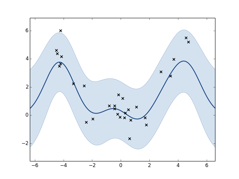
Plot of the GP model before optimization. Black x’s are training points. The line is the predicted function (posterior mean). The shaded region corresponds to the roughly 95% confidence interval.
m.optimize()
print m
m.plot()
Name : GP regression
Log-likelihood : -13.3897302116
Number of Parameters : 3
Parameters:
GP_regression. | Value | Constraint | Prior | Tied to
rbf.variance | 465.887938367 | +ve | |
rbf.lengthscale | 10.2848156804 | +ve | |
Gaussian_noise.variance | 0.0488157865927 | +ve | |
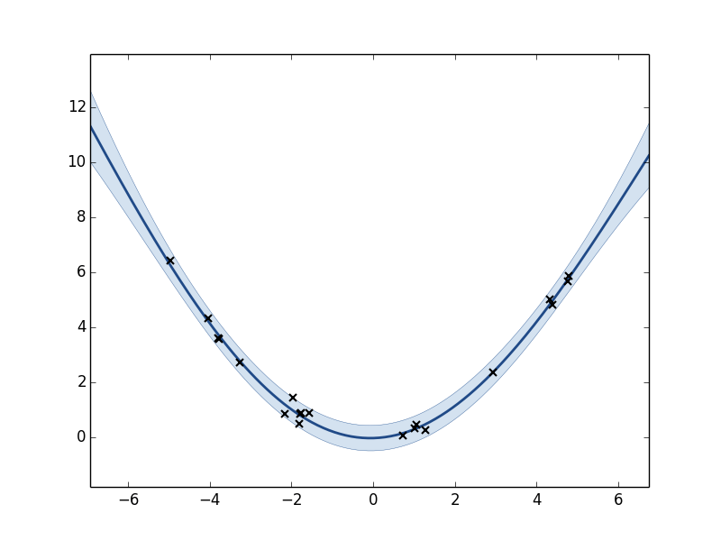
Plot of the GP model after optimization.
After the parameters of the model have been optimized the GP has a significant better fit on the underlying function. We can see that all parameter values have changed from their default values.
Alternatives
There are also other GP frameworks for python apart from GPy. The pyGPs (docs) package is a good example with support for both classification and regression.
References
We follow here the definitions as described by Rasmussen, C. E., & Williams, C. (2006). Gaussian Processes for Machine Learning. the MIT Press. ↩︎