Prostate cancer (PCa) is the one of the most common cancers in the world1 and is graded by pathologist using the Gleason grading system. The grading system was originally made by correlating distinctive patterns in the tissue to patient survival:
“The way to develop a histologic classification was to forget anything I thought I knew about the behavior of prostate cancer and simply look for different histologic pictures … . Then, the pictures would be handed to statisticians and compared with a ‘gold standard’ of clinical tumor behavior (ie, patient survival).” - Donald F. Gleason
As an AI scientist, to me this sounds a lot like pattern recognition; something computers could potentially do better. Currently the grading system consists of 5 distinct classes (of which practically only 3 are used), who says that there are not 10 or 50 relevant morphological classes in the data? That is why I am interested in unsupervised methods that can extract patterns from data and want to apply this to detecting and grading prostate cancer. All information is already present in the data, we ‘just’ need to find methods to retrieve it.
Overview of the method (Click for larger version)
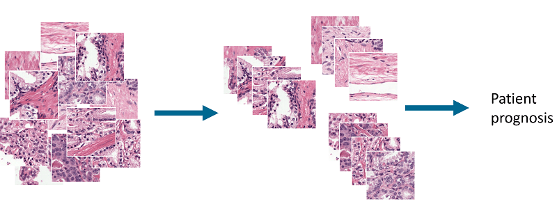
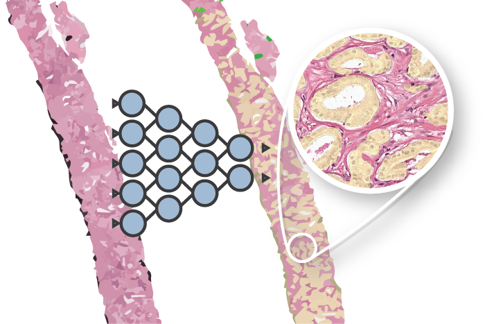
At MIDL2018 I presented a first step towards this goal: an unsupervised method for detecting and grading prostate cancer. The idea behind this project is to cluster prostate tissue in an unsupervised fashion and then later link these clusters to patient prognosis.

Overview of the idea. By clustering patches of prostate tissue we can make groups that can be used to classify tissue and used for patient prognosis.
Methods overview
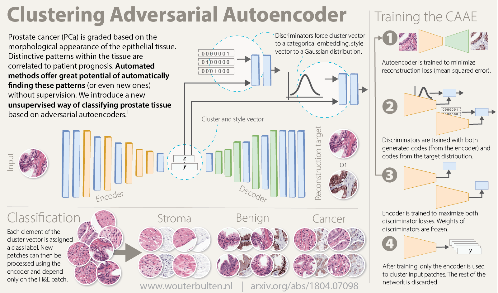
Our method is based on adversarial autoencoders and uses these autoencoders to cluster tissue during training: a clustering adversarial autoencoder (CAAE)2. As opposed to normal autoencoders, this method does not require post-processing in terms of kMeans, t-SNE or other clustering methods.
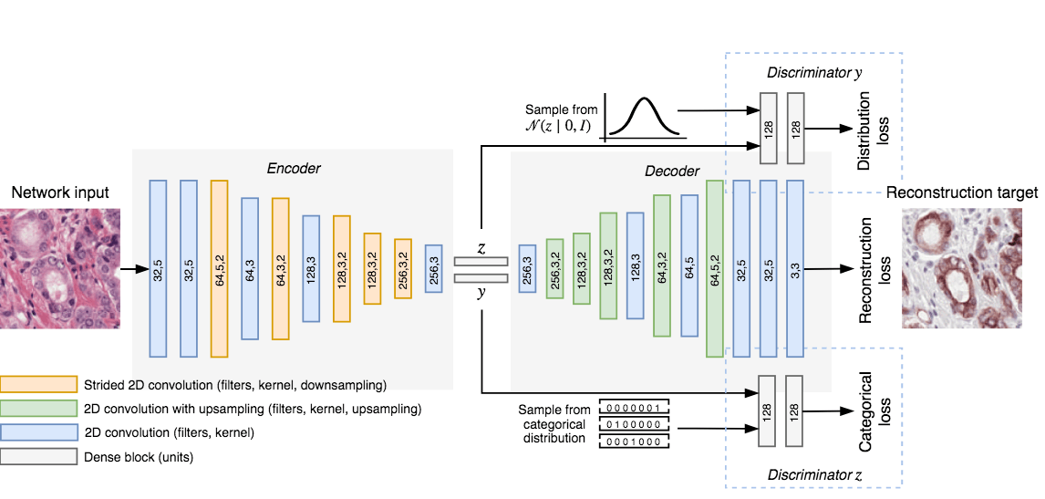
Overview of network topology. The network reconstructs an IHC patch from an H&E patch using two vectors: the cluster vector y and a style vector z. A different reconstruction target domain forces the network to learn more relevant features.
Our CAAE consists of four subnetworks (see figure above) and two latent vectors as the embedding. The first latent vector, y (size 50), represents the cluster vector and is regularized by a discriminator to follow a one-hot encoding. This is the vector that is used for the clustering and represent high level structures in the data (for example, in case of MNIST this could represent individual digits). The second latent vector, z (size 20), represents the style of the input patch, and follows a Gaussian distribution (think of writing style in MNIST).
Training the CAAE forces the network to describe high level information in the cluster vector using one of the 50 classes, and low-level reconstruction information in the style vector. The ratio between the length of the two vectors is critical, a too large z and the network will encode all information using the more easy to encode style vector and disregard the cluster vector.
The CAAE is trained in three stages on each minibatch. First, the autoencoder itself is updated to minimize the reconstruction loss. Second, both discriminators are updated to regularize y and z using data from the encoder and the target distribution. Last, the adversarial part is trained by connecting the encoder to the two discriminators separately and maximizing the individual discriminator loss, updating only the encoder’s weights. This forces the latent spaces to follow the target distributions.
Data & Anti-body driven feature learning
We trained our CAAE on patches (128 x 128 pixels) extracted from registered whole slide image (WSI) pairs. Each pair consists of a H&E slide (the staining method that is used for grading prostate cancer), and a slide that was processed using immunohistochemistry (IHC) with an epithelial (CK8/18) and basal cell (P63) marker. The patches were sampled at random as no annotations or information regarding tumor location was available.
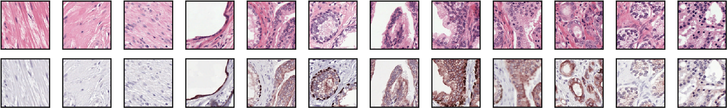
Examples from the dataset.
The H&E patches were used as training input. We tested two reconstruction targets: using the input patch as the target (H&E to H&E) and using the IHC version of the same patch (H&E to IHC). By using a IHC patch as reconstruction target we force the network to learn which features in H&E correspond to features in the IHC; we hypothesized that this anti-body driven feature learning results in more relevant encodings as the network needs to learn which features in the H&E correspond to features in IHC.
Results
After training the networks can be used to cluster new patches by passing patches through the encoder. The other components of the network can be discarded. By taking the argmax of the cluster vector each patch is assigned to a single cluster. A few examples clusters are shown below. Note that not every cluster is relevant as we enforce no structure or prior knowledge on the clustering.
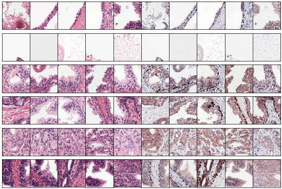
Example clusters. Some clusters capture a class perfectly, e.g. stroma in row 1 and 2 and tumor in row 5. Some clusters look similar but contain both benign epithelium and tumor (row 6).
The best network achieves an F1 score of 0.62 on tumor versus non-tumor (see paper for all experiments and results). This score leaves enough room for improvement, but our network achieves this score without using labeled training data on a very noise dataset. In other words, lots of work still ahead of us but it shows that there is information in the data that we can extract using these autoencoders. Donwsides of this method are that these autoencoders are hard to train, can suffer from mode collapse (i.e. only 1 cluster is formed) and can be very unstable during training.
To determine whether the clustering encodes relevant information we can, for visualisation, apply the network as a sliding window to a larger area. Of course this is not really useful for diagnostics, as it is very coarse, but it gives an overview of what the network ‘sees’. This method results in nice heatmaps for each class:
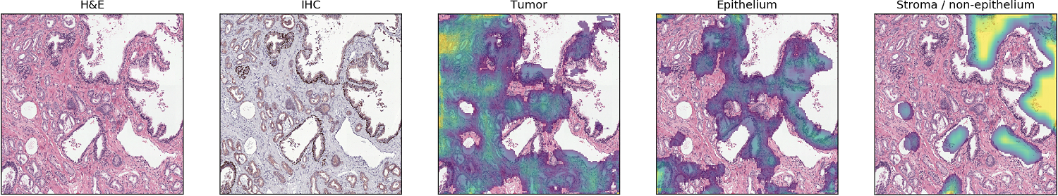
Network applied as a sliding window.
More info & citation
This work was presented at MIDL 2018. Want to read more? Please refer to the conference abstract as it contains more detail on the data, training procedure and network architectures. Feel free to add any questions as comments to this post.
You can use the following reference if you want to cite my paper:
W. Bulten and G. Litjens. “Unsupervised Prostate Cancer Detection on H&E using Convolutional Adversarial Autoencoders”, in: Medical Imaging with Deep Learning, 2018
Or, if you prefer BibTeX:
@InProceedings{Bulten18,
  author    = {Bulten, Wouter and Litjens, Geert},
  title     = {Unsupervised Prostate Cancer Detection on H\&E using Convolutional Adversarial Autoencoders},
  booktitle = {Medical Imaging with Deep Learning},
  year      = {2018},
  url       = {https://arxiv.org/abs/1804.07098},
  abstract  = {We propose an unsupervised method using self-clustering convolutional adversarial autoencoders to classify prostate tissue as tumor or non-tumor without any labeled training data. The clustering method is integrated into the training of the autoencoder and requires only little post-processing. Our network trains on hematoxylin and eosin (H\&E) input patches and we tested two different reconstruction targets, H&E and immunohistochemistry (IHC). We show that antibody-driven feature learning using IHC helps the network to learn relevant features for the clustering task. Our network achieves a F1 score of 0.62 using only a small set of validation labels to assign classes to clusters.},
}
Series on my PhD in Computational Pathology
This post is part of a series related to my PhD project on prostate cancer, deep learning and computational pathology. In my research I developed AI algorithms to diagnose prostate cancer. Interested in the rest of my research? The three latest post are shown below. For all the posts, you can find all posts tagged with research.
Latest post related to my research
AI for diagnosis of prostate cancer: the PANDA challenge
Artificial intelligence (AI) for prostate cancer analysis is ready for clinical implementation, shows a global programming competition, the PANDA challenge.
Improve prostate cancer diagnosis: participate in the PANDA Gleason grading challenge
Can you build a deep learning model that can accurately grade protate biopsies? Participate in the PANDA challenge
The potential of AI in medicine: AI-assistance improves prostate cancer grading
In a completely new study we investigated the possible benefits of an AI system for pathologists. Instead of focussing on pathologist-versus-AI, we instead look at potential pathologist-AI synergy.
Deep learning posts
Sometimes I write a blog post on deep learning or related techniques. The latest posts are shown below. Interested in reading all my blog posts? You can read them on my tech blog.
Simple and efficient data augmentations using the Tensorfow tf.Data and Dataset API
The tf.data API of Tensorflow is a great way to build a pipeline for sending data to the GPU. In this post I give a few examples of augmentations and how to implement them using this API.
Getting started with GANs Part 2: Colorful MNIST
In this post we build upon part 1 of 'Getting started with generative adversarial networks' and work with RGB data instead of monochrome. We apply a simple technique to map MNIST images to RGB.
Getting started with generative adversarial networks (GAN)
Generative Adversarial Networks (GANs) are one of the hot topics within Deep Learning right now and are applied to various tasks. In this post I'll walk you through the first steps of building your own adversarial network with Keras and MNIST.
References
Torre, L. A., Bray, F., Siegel, R. L., Ferlay, J., Lortet-tieulent, J., and Jemal, A., “Global Cancer Statistics, 2012,” CA: a cancer journal of clinicians. 65(2), 87-108 (2015). ↩︎
A. Makhzani, J. Shlens, N. Jaitly, and I. Goodfellow, “Adversarial autoencoders,” in International Conference on Learning Representations, 2016. ↩︎