Recently, I presented a conference article at SPIE Medical Imaging 2018, as part of my PhD in computational pathology, deep learning and prostate cancer. In this project we tackled the problem of epithelium segmentation using deep learning. It was the first project I worked on within computational pathology.
This post gives a highlight of our work. Want to have more in depth details? All details on the data, training procedure and network architectures are available in the article itself.
Why epithelium?
Prostate cancer (PCa) is the most common cancer in men in developed countries1. PCa develops from genetically damaged glandular epithelium and in the case of high-grade tumors, the glandular structure is eventually lost2. As PCa originates from epithelial cells, glandular structures within prostate specimens are regions of interest for finding malignant tissue.
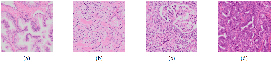
Different types of glands: normal glandular structure (a); poorly differentiated, high-grade Gleason 5 PCa (b); non-tumor epithelium surrounded by inflammation (c); Gleason 3 PCa showing color variation between slides (d).
Building systems to detect tumor is often hard due to a lack of data. In general, more data equals a higher performance. Typically, deep learning methods that try to detect cancer from scanned tissue specimens use a set of annotated cancer regions as the reference standard for training. As these algorithms learn from their training data, the quality of the annotations directly influences the quality of the output. Tumor annotations made by pathologists are often coarse due to time constraints (see picture below, 2nd image). Outlining all individual tumor cells within PCa is practically infeasible due to the mixture of glandular, stromal and inflammatory components. These coarse annotations limit the potential of these deep learning methods.
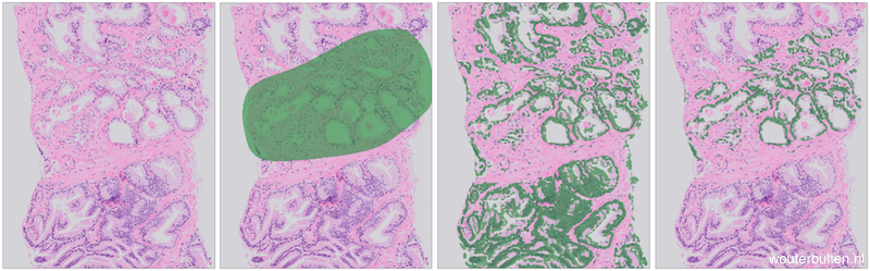
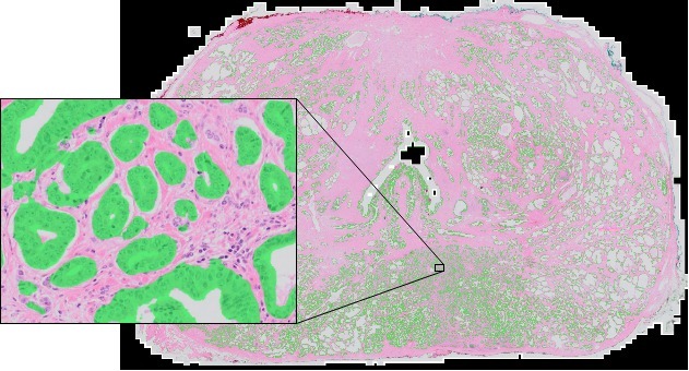
Example prostate tissue with PCa (extracted from a core needle biopsy) (1), tumor annotations (2), epithelium segmentation (3), segmentation and annotations combined (4).
We propose a method to automatically refine these coarse tumor annotations by training a system that can automatically filter out irrelevant parts of the data, in this case all non-epithelial tissue. This method results in fine-grained annotations without additional manual effort.
How did we approach this?
As data for our experiments we used 30 digitally scanned H&E whole mount tissue sections from 27 patients that underwent RP treatment. The reported Gleason growth patterns in these sections ranged from 3 to 5. The specimens were randomly split into three sets: 15 slides for training, 5 for validation and 10 for testing.
We compared U-Net3 (which is specifically designed for segmentation) and a general fully convolutional network (FCN). For both types of network we tested differences in layer depth. The networks are trained on patches extracted from digitally scanned prostate tissue slices at 10x magnification.
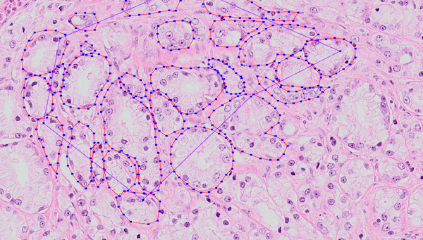
Example of annotated training data. Many of these regions were annotated by hand. The annotated epithelial glands are outlined in red.
What are the results?
The most important numerical results can be found in the table below. See the article for a breakdown in cancer/non-cancer.
For both types of networks, the deeper the network the higher the performance. However, a deeper network also increases the parameter complexity, especially in the case of the FCN. Given the comparable performance, we labeled the U-Net as the winner given its lower parameter count.
The best U-Net produces fine grained segmentations and achieves a F1 score of 0.82 and an AUC of 0.97.
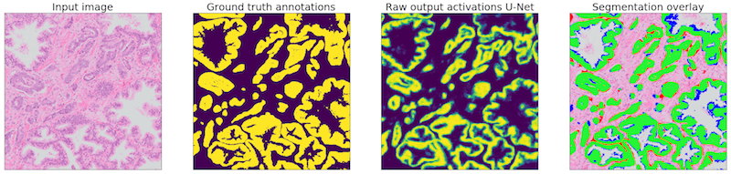
Example of one of the regions of our test set. The network is applied to the input image (1). The ground truth (2) can then be compared with the network output (3). The segmentation overlay (4) shows the performance of the network: green marked pixels show true positive, blue false negative and red false positive.
| Network | Depth | Contraction parameters | Total parameters | F1 | Accuracy | AUC total | |
|---|---|---|---|---|---|---|---|
| 1 | U-Net | 2 | 16,944 | 26,130 | 0.79 | 0.87 | 0.95 |
| 2 | U-Net | 3 | 72,752 | 118,162 | 0.82 | 0.90 | 0.96 |
| 3 | U-Net | 4 | 294,960 | 484,498 | 0.82 | 0.90 | 0.97 |
| 4 | FCN | 2 | 16,944 | 6,322,738 | 0.79 | 0.87 | 0.94 |
| 5 | FCN | 3 | 72,752 | 10,572,850 | 0.81 | 0.88 | 0.95 |
| 6 | FCN | 4 | 294,960 | 19,183,666 | 0.83 | 0.89 | 0.96 |
Next steps
Room for improvement lays with segmenting glands as a whole. Our models rarely misses complete cancer regions, though with some high-grade PCa only parts of the glands are detected. We suspect that most of the errors are, first of all, caused by a lack of training examples and not due to a limitation of the models.
A logical next step is to improve our dataset. However, manual annotations are flawed due to the difficulty of making correct and precise annotations, especially in tumor areas. A potential solution for this is using immunohistochemistry to assist in making annotations. By using specific stains that highlight epithelial cells, we hope to generate precise and less erroneous annotations of epithelial tissue.
After training the networks can be applied on a whole-slide level, segmenting the full prostate slide. Each slide is extremely large and measures around 200.000 by 100.000 pixels.
More info & citation
This work was presented at SPIE Medical Imaging 2018. Want to read more? Please refer to the conference paper as it contains more detail on the data, training procedure and network architectures. Feel free to add any questions as comments to this post.
You can use the following reference if you want to cite my paper:
Wouter Bulten, Christina A. Hulsbergen-van de Kaa, Jeroen van der Laak, Geert J. S. Litjens, “Automated segmentation of epithelial tissue in prostatectomy slides using deep learning,” Proc. SPIE 10581, Medical Imaging 2018: Digital Pathology, 105810S (6 March 2018)
Or, if you prefer BibTeX:
@inproceedings{Bulten2018,
  author = {Bulten, Wouter and {Hulsbergen-van de Kaa}, Christina A. and van der Laak, Jeroen and Litjens Geert J S},
  booktitle = {Medical Imaging 2018: Digital Pathology},
  doi = {10.1117/12.2292872},
  isbn = {9781510616516},
  title = {{Automated segmentation of epithelial tissue in prostatectomy slides using deep learning}},
  volume = {10581},
  year = {2018}
}
Series on my PhD in Computational Pathology
This post is part of a series related to my PhD project on prostate cancer, deep learning and computational pathology. In my research I developed AI algorithms to diagnose prostate cancer. Interested in the rest of my research? The three latest post are shown below. For all the posts, you can find all posts tagged with research.
Latest post related to my research
AI for diagnosis of prostate cancer: the PANDA challenge
Artificial intelligence (AI) for prostate cancer analysis is ready for clinical implementation, shows a global programming competition, the PANDA challenge.
Improve prostate cancer diagnosis: participate in the PANDA Gleason grading challenge
Can you build a deep learning model that can accurately grade protate biopsies? Participate in the PANDA challenge
The potential of AI in medicine: AI-assistance improves prostate cancer grading
In a completely new study we investigated the possible benefits of an AI system for pathologists. Instead of focussing on pathologist-versus-AI, we instead look at potential pathologist-AI synergy.
Deep learning posts
Sometimes I write a blog post on deep learning or related techniques. The latest posts are shown below. Interested in reading all my blog posts? You can read them on my tech blog.
Simple and efficient data augmentations using the Tensorfow tf.Data and Dataset API
The tf.data API of Tensorflow is a great way to build a pipeline for sending data to the GPU. In this post I give a few examples of augmentations and how to implement them using this API.
Getting started with GANs Part 2: Colorful MNIST
In this post we build upon part 1 of 'Getting started with generative adversarial networks' and work with RGB data instead of monochrome. We apply a simple technique to map MNIST images to RGB.
Getting started with generative adversarial networks (GAN)
Generative Adversarial Networks (GANs) are one of the hot topics within Deep Learning right now and are applied to various tasks. In this post I'll walk you through the first steps of building your own adversarial network with Keras and MNIST.
References
Torre, L. A., Bray, F., Siegel, R. L., Ferlay, J., Lortet-tieulent, J., and Jemal, A., “Global Cancer Statistics, 2012,” CA: a cancer journal of clinicians. 65(2), 87-108 (2015). ↩︎
Fine, S. W., Amin, M. B., Berney, D. M., Bjartell, A., Egevad, L., Epstein, J. I., Humphrey, P. A., Magi- Galluzzi, C., Montironi, R., and Stief, C., “A contemporary update on pathology reporting for prostate cancer: Biopsy and radical prostatectomy specimens,” European Urology 62(1), 20–39 (2012). ↩︎
Ronneberger, O., Fischer, P., & Brox, T. (2015, October). U-net: Convolutional networks for biomedical image segmentation. In International Conference on Medical image computing and computer-assisted intervention (pp. 234-241). Springer, Cham. ↩︎