In the previous post I talked about getting started with generative adversarial networks (GANs) and applied these types of networks to the MNIST dataset. In that application we limited ourselves to 1D black-and-white images which are fairly easy for a network to learn. Eventually though, we want to switch to more complex (RGB) images. In this post I discuss a way of enhancing the MNIST dataset with colors, a colorful MNIST so to say.
This new generated dataset is a convenient way to start with generating RGB images and acts as a nice stepping stone for working with GANs in combination with more difficult datasets. In fact, for my own research I used this method to get some hands on experience with generating RGB images before applying GANs on my own data.
If your not familiar with GANs and/or want to read a more introductionary article. Please see my “getting started with GANs” post.
All the code, including code for making the figures, can be found in my deep learning resources GitHub repository.
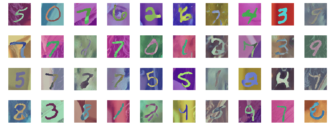
Example images from the MNIST dataset mixed with generated images. The real images are mapped to the RGB space, the fake images are directly from the output oft the generator.
Loading the data
Same as before, we start with reading the original MNIST data. For this I use a small utility function from Tensorflow. The MNIST set is later used as a base for generating our colorfull images.
# Read MNIST data
x_train = input_data.read_data_sets("mnist", one_hot=True).train.images
x_train = x_train.reshape(-1, 28, 28, 1).astype(np.float32)
With the MNIST images loaded we are going to map these to a 3-channel space by adding color. The resulting images are in RGB and will be more difficult for the network to train. Nevertheless, the complexity of the images is still manageable and these images can still be generated by a fairly simple GAN. This makes it a perfect next step after working on the black-and-white images.
We cannot just add random colored noise to the image because we want our generator the learn a certain structure. Therefor I apply a nice technique I adapted from a repository on domain adaptation. The main idea is to blend a MNIST digit with a colorful background to generate a new image in RGB space. As the background I use the popular “Lenna” or “Lena” image, but any other image can be used.
# Read Lena image
lena = PILImage.open('resources/lena.jpg')
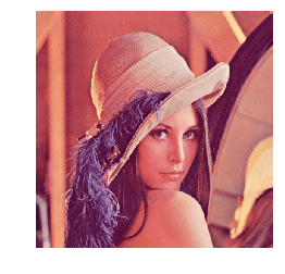
The Lena image
To generate a new sample we start with taking a random crop of the Lena image; this will be used as the background. Then, for every pixel of the MNIST digit we invert the colors to show the original number. To make the examples a bit more detailed we also upsample the digits to 64x64 pixels.
def get_mnist_batch(batch_size=256, change_colors=True):

    # Select random batch (WxHxC)
    idx = np.random.choice(x_train.shape[0], batch_size)
    batch_raw = x_train[idx, :, :, 0].reshape((batch_size, 28, 28, 1))

    # Resize (this is optional but results in a training set of larger images)
    batch_resized = np.asarray([scipy.ndimage.zoom(image, (2.3, 2.3, 1), order=1) for image in batch_raw])

    # Extend to RGB
    batch_rgb = np.concatenate([batch_resized, batch_resized, batch_resized], axis=3)

    # Convert the MNIST images to binary
    batch_binary = (batch_rgb > 0.5)

    # Create a new placeholder variable for our batch
    batch = np.zeros((batch_size, 64, 64, 3))

    for i in range(batch_size):
        # Take a random crop of the Lena image (background)
        x_c = np.random.randint(0, lena.size[0] - 64)
        y_c = np.random.randint(0, lena.size[1] - 64)
        image = lena.crop((x_c, y_c, x_c + 64, y_c + 64))
        # Conver the image to float between 0 and 1
        image = np.asarray(image) / 255.0

        if change_colors:
            # Change color distribution
            for j in range(3):
                image[:, :, j] = (image[:, :, j] + np.random.uniform(0, 1)) / 2.0

        # Invert the colors at the location of the number
        image[batch_binary[i]] = 1 - image[batch_binary[i]]

        batch[i] = image

    return batch
A set of example images is shown below:
count = 20
examples = get_mnist_batch(count)

plt.figure(figsize=(15,3))
for i in range(count):
    plt.subplot(2, count // 2, i+1)
    plt.imshow(examples[i])
    plt.axis('off')

plt.tight_layout()
plt.show()
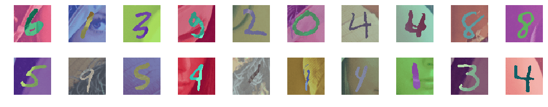
20 randomly selected training images
Defining the network
Now that we have created our new dataset we can define the network. As with most GANs, this network consists of a discriminator and a generator. Please see the previous post for more information about their role. I adapted the network used in that post to work with RGB images. The discriminator has a 64x64x3 input vector and outputs a single digit. The generator uses a 100x1 noise vector to generate 64x64x3 sized images.
def discriminator():

    net = Sequential()
    input_shape = (64, 64, 3)
    dropout_prob = 0.4

    net.add(Conv2D(64, 5, strides=2, input_shape=input_shape, padding='same'))
    net.add(LeakyReLU())

    net.add(Conv2D(128, 5, strides=2, padding='same'))
    net.add(LeakyReLU())
    net.add(Dropout(dropout_prob))

    net.add(Conv2D(256, 5, strides=2, padding='same'))
    net.add(LeakyReLU())
    net.add(Dropout(dropout_prob))

    net.add(Conv2D(512, 5, strides=2, padding='same'))
    net.add(LeakyReLU())
    net.add(Dropout(dropout_prob))

    net.add(Flatten())
    net.add(Dense(1))
    net.add(Activation('sigmoid'))

    return net
def generator():

    net = Sequential()
    dropout_prob = 0.4

    net.add(Dense(8*8*256, input_dim=100))
    net.add(BatchNormalization(momentum=0.9))
    net.add(Activation('relu'))
    net.add(Reshape((8,8,256)))
    net.add(Dropout(dropout_prob))

    net.add(UpSampling2D())
    net.add(Conv2D(128, 5, padding='same'))
    net.add(BatchNormalization(momentum=0.9))
    net.add(Activation('relu'))

    net.add(UpSampling2D())
    net.add(Conv2D(128, 5, padding='same'))
    net.add(BatchNormalization(momentum=0.9))
    net.add(Activation('relu'))

    net.add(UpSampling2D())
    net.add(Conv2D(64, 5, padding='same'))
    net.add(BatchNormalization(momentum=0.9))
    net.add(Activation('relu'))

    net.add(Conv2D(32, 5, padding='same'))
    net.add(BatchNormalization(momentum=0.9))
    net.add(Activation('relu'))

    net.add(Conv2D(3, 5, padding='same'))
    net.add(Activation('sigmoid'))

    return net
optim_discriminator = RMSprop(lr=0.0002, clipvalue=1.0, decay=6e-8)
model_discriminator = Sequential()
model_discriminator.add(net_discriminator)
model_discriminator.compile(loss='binary_crossentropy', optimizer=optim_discriminator, metrics=['accuracy'])
optim_adversarial = Adam(lr=0.0001, clipvalue=1.0, decay=3e-8)
model_adversarial = Sequential()
model_adversarial.add(net_generator)

# Disable layers in discriminator
for layer in net_discriminator.layers:
    layer.trainable = False

model_adversarial.add(net_discriminator)
model_adversarial.compile(loss='binary_crossentropy', optimizer=optim_adversarial, metrics=['accuracy'])
Training the networks
For brevity the whole training code is not shown here as it contains many functions for plotting and monitoring. Please see the repository for the an annotated Jupyter notebook containing all the Python code. The code below shows the minimal example needed for training:
for i in range(0, 20001):

    # Select a random set of training images from the new dataset
    images_train = get_mnist_batch(batch_size)
    # Generate a random noise vector
    noise = np.random.uniform(-1.0, 1.0, size=[batch_size, 100])
    # Use the generator to create fake images from the noise vector
    images_fake = net_generator.predict(noise)

    # Create a dataset with fake and real images
    x = np.concatenate((images_train, images_fake))
    y = np.ones([2*batch_size, 1])
    y[batch_size:, :] = 0

    # Train discriminator for one batch
    d_stats = model_discriminator.train_on_batch(x, y)

    # Train the generator
    # The input of th adversarial model is a list of noise vectors. The generator is 'good' if the discriminator classifies
    # all the generated images as real. Therefore, the desired output is a list of all ones.
    y = np.ones([batch_size, 1])
    noise = np.random.uniform(-1.0, 1.0, size=[batch_size, 100])
    a_stats = model_adversarial.train_on_batch(noise, y)
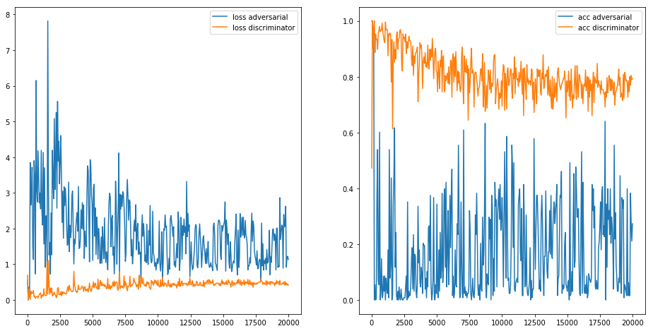
The loss (left) and accuracy (right) graphs of both the discriminator and the generator using training. The whole network was trained for 20.000 iterations.
By applying the generator during training on the same noise vector we can visualize how the generator trains. Below is a movie of the generator output at every 100 iterations:
Wrapping up
In this post we looked at an easy way to start with generating RGB images with GANs. This was meant as a small step-up from generating monochrome images. In the image below real and fake images are combined:
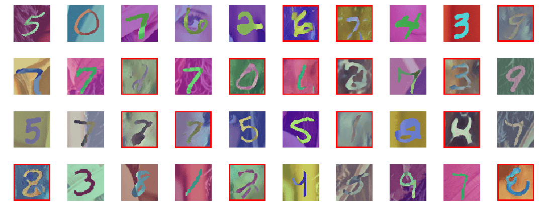
Both real and fake digits combined in the same image. Red outlined digits are generated by the adversarial network.
The generated images are not as good as in the black-and-white example, this is mainly caused by the difficult training set. With this new dataset the generator must not only generate digits but als a valid background (which is retrieved from a real image). With more training or some special techniques you can probably improve these generated images. But, as this was a way of getting used to RGB images with GANs I was very pleased with the results. Please let me know (in the comments below) if you have any nice results or ideas to improve the generated images. I would gladly hear your thoughts!
The full source code of this post is available as a Jupyter notebook and can be found in my deep learning resource repository.

Playing around with the noise vector shows that it encodes both the digits as the background.